Lecture 10
MAP, MLE, and Score Function
$$
$$
Gradient Descent with Score Function
The classic inverse problem is defined as
\[b = F(x) + \epsilon\]
where \(F(x)\) is the forward operator, \(b\) is the observed data, and \(\epsilon\) represents the noise in the measurement or process. We often assume that \(\epsilon\) is Gaussian with zero mean and covariance matrix \(\Sigma\).
\[ \epsilon \sim \mathcal{N}(0, \Sigma) \]
The probability density of the deviation of the observed data from the forward model in this case is given by: \[ \pi(\epsilon) = \frac{1}{(2\pi)^{m/2}|\Sigma|^{1/2}} \exp\left(-\frac{1}{2}\epsilon^\intercal \Sigma^{-1} \epsilon\right) \]
Without any prior information about the error, it is difficult to estimate the covariance matrix \(\Sigma\). For the purpose of this analysis we can assume that it is a normal distribution with zero mean and a diagonal \(\sigma^2 I\) covariance matrix. The likelihood function then simplifies to:
\[ \pi(\epsilon) = \frac{1}{(2\pi \sigma^2)^{m/2}} \exp\left(-\frac{1}{2\sigma^2}\|b-F(x)\|^2 \right) \]
To model the probability distribution of the inverse problem parameters \(x\), we introduce a prior distribution \(\pi(x)\). To ensure positivity of \(\pi(x)\) over the entire domain and proper normalization, we define it using a potential function \(\phi(x, \theta)\): \[\pi(x; \theta) = \frac{e^{-\phi(x, \theta)}}{Z(\theta)}\]
where the partition function \(Z(\theta)\) is given by:
\[Z(\theta) = \int_\Omega e^{-\phi(x, \theta)} dx\]
Note that the partition function is required to make the probability distribution integrate to \(1\). The exponential operator on the potential ensures that all \(\pi(x)\) values are positive, since \(e^{-\phi} > 0\) for all \(\phi \in \mathbb{R}\). In practice, it is often intractable to directly compute the partition function when updating the model parameters \(\theta\) for distributions more complex than a Gaussian.
\(\phi(x, \theta): \mathbb{R}^n \rightarrow \mathbb{R}\) maps \(x\) to a scalar value, and \(\theta\) are the parameters of the model. For example, if we are modeling a Gaussian, the parameters might include the covariance matrix \(\Sigma\). The potential has a physical interpretation as the energy of a system, where high \(\phi\) values correspond to low probability density regions. For this reason it is often called the energy function in physics-inspired models.
Maximum A Posteriori Estimation
The goal of maximum a posteriori (MAP) estimation is to find the most likely \(x\) given the observed data \(b\) and model parameters \(\theta\), by maximizing the posterior probability \(\pi(x|b; \theta)\):
\[ \begin{align*} \max_x \pi(x|b; \theta) &= \max_x \frac{\pi(b|x; \theta) \pi(x; \theta)}{\pi(b)}\\ \max_x \underbrace{\pi(x|b; \theta)}_{\text{Posterior}} & = \max_x \underbrace{\pi(b|x; \theta)}_{\text{Likelihood}} \underbrace{\pi(x; \theta)}_{\text{Prior}}\\ \end{align*} \]
Since \(\pi(b)\) is independent of \(x\), it does not affect the maximization problem. Substituting the likelihood and prior distributions, we have:
\[ \begin{align*} & = \max_x \frac{1}{(2\pi \sigma^2)^{m/2}} \exp\left(-\frac{1}{2\sigma^2}\|b-F(x)\|^2 \right) \frac{1}{Z(\theta)} e^{-\phi(x, \theta)} \end{align*} \]
The logarithm is a monotonic function, so we can maximize the log of the posterior instead of the posterior itself with no loss of generality: \(\arg\max_x \pi(x) = \arg\max_x \log(\pi(x))\). Intuitively, since the logarithm is always increasing, \(\log(z) > \log(y)\) implies \(z > y\). In addition, the log of a product of exponentials is the sum of the exponents, and the maximum of a function is the minimum of its negative. This allows us to rewrite the objective as:
We have previously looked at methods for differentiating the forward operator \(F\) and performing gradient descent. We take the gradient with respect to \(x\) to find the minimum of the function:
\[ \begin{align*} g &= \nabla_x \left(\frac{1}{2\sigma^2}\|b-F(x)\|^2 + \phi(x, \theta)\right)\\ &= \frac{1}{\sigma^2} J^T(x) (F(x) - b) + \nabla_x \phi(x, \theta)\\ &= \frac{1}{\sigma^2} J^T(x) (F(x) - b) - s(x, \theta) \end{align*} \]
Using gradient descent, we can update the estimate of \(x\) by taking steps away from the direction of the gradient \(g\):
\[x_{k+1} = x_k - \alpha g\]
Score Function
\(s(x;\theta)\) is known as the score function of \(\pi(x; \theta)\): \[s(x, \theta):= \nabla_x \log (\pi(x; \theta)) = - \nabla_x \phi(x, \theta)\]
where the \(\log Z(\theta)\) term vanishes because it does not depend on \(x\). The score is the negative gradient of the potential function \(\phi(x, \theta)\) with respect to \(x\). The score function generalizes the gradient of the log-likelihood function, and is described in more detail in Schervish’s “Theory of Statistics” (Schervish 1995).
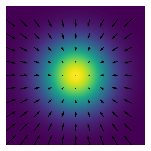
Score has a physical intuition connected to energy potentials and fields. In physics, the electric field \(\mathbf{E}\) is the negative gradient of the electric potential \(V\): \[ \mathbf{E} = -\nabla_x V(x)\]
Similarly, the score function is the negative gradient of the potential function \(\phi(x, \theta)\) in the case where \(\pi(x) \propto e^{-\phi(x, \theta)}\). The score function points in the direction of steepest increase of the log probability density.
Example: 2D Gaussian Distribution
Consider a 2D Gaussian distribution with zero mean and covariance \(\sigma^2 I\):
| Function | Expression |
|---|---|
| Probability Distribution | \(\pi(x) = \frac{1}{2\pi \sigma^2}\exp\left( -\frac{1}{2\sigma^2} \| x \|^2 \right)\) |
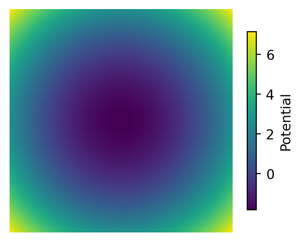
| Potential Function | \(\phi(x, \theta) = \frac{1}{2\sigma^2} \| x \|^2 + \log(2\pi \sigma^2)\) |
| Score Function | \(s(x, \theta) = -\nabla_x \phi(x, \theta) = -\frac{x}{\sigma^2}\) |
In regions of high probability density, the potential function is low, because the relation \(\pi(x) = e^{-\phi(x, \theta)}\) is monotonically decreasing in \(\phi(x, \theta)\). The score function always points in the local direction of steepest increase of the log probability density — here, towards the center of the Gaussian.
Visualization
Below is a visualization of the probability density function (PDF), potential function, and score function of a 2D Gaussian distribution.
Show the code
import numpy as np
import matplotlib.pyplot as plt
import seaborn as sns

# Make plots for a 2D Gaussian distribution heatmap, potential function, and score function

# Define the 2D Gaussian distribution
def gaussian_pdf(x, y, sigma=1):
    return np.exp(-0.5*(x**2 + y**2)/sigma**2)/(2*np.pi*sigma**2)

# Define the potential function
def potential_function(x, y, sigma=1):
    return 0.5*(x**2 + y**2)/sigma**2 + np.log(2*np.pi*sigma**2)

# Define the score function
def score_function(x, y, sigma=1):
    return -np.array([x, y])/sigma**2

# Create a grid of points
x = np.linspace(-3, 3, 500)
y = np.linspace(-3, 3, 500)
X, Y = np.meshgrid(x, y)

# Compute the PDF, potential function, and score function
pdf = gaussian_pdf(X, Y)
potential = potential_function(X, Y)
score = score_function(X, Y)

# Plot the Probability Distribution with a colorbar
plt.figure(figsize=(4, 3))
im = plt.imshow(pdf, cmap='viridis', extent=[-3, 3, -3, 3])
plt.axis('off')
plt.colorbar(im, shrink=0.8, label="Density")
plt.show()

# Plot the Potential Function with a colorbar
plt.figure(figsize=(4, 3))
im = plt.imshow(potential, cmap='viridis', extent=[-3, 3, -3, 3])
plt.axis('off')
plt.colorbar(im, shrink=0.8, label="Potential")
plt.show()

# Downsample the grid for quiver plotting
step = 50  # Downsample by taking every 50th point
X_downsampled = X[::step, ::step]
Y_downsampled = Y[::step, ::step]
score_downsampled = score_function(X_downsampled, Y_downsampled)

# Plot the Score Function as a quiver plot over the PDF
plt.figure(figsize=(4, 3))
plt.imshow(pdf, cmap='viridis', extent=[-3, 3, -3, 3])
plt.quiver(
    X_downsampled, Y_downsampled,
    score_downsampled[0], score_downsampled[1],
    color='black'
)
plt.axis('off')

# Save to file
plt.savefig("imgs/score_function.png", bbox_inches='tight')

plt.show()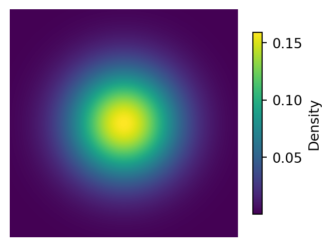
Maximum Likelihood Estimate from Samples
A common problem is estimating a probability distribution \(\pi(x)\) based on a set of empirical samples \(\{x_1, x_2, ..., x_N\}\). Often in statistical analysis, we are working with an unknown \(\pi\) and attempting to make our best estimate from sampled data. If we assume that the drawn samples are independent and identically distributed (i.i.d.), then the likelihood of the samples is the product of the likelihoods of each sample. Recalling that \(Z(\theta) = \int_\Omega e^{-\phi(x, \theta)} dx\), the likelihood of the samples is:
\[ \begin{align*} \pi(x_1, x_2, ..., x_N) &= \prod_{i=1}^N \pi(x_i) = \pi(x_1) \pi(x_2) ... \pi(x_N) \\ &= \frac{1}{Z(\theta)} \exp\left(-\phi(x_1, \theta)\right) \frac{1}{Z(\theta)} \exp\left(-\phi(x_2, \theta)\right) ... \frac{1}{Z(\theta)} \exp\left(-\phi(x_N, \theta)\right) \\ &= \frac{1}{\left[Z(\theta)\right]^N} \exp\left(-\sum_{i=1}^N \phi(x_i, \theta)\right) \end{align*} \]
Since some \(x\) are observed, the challenge is to find the potential function \(\phi(x, \theta)\) that maximizes the likelihood of the samples, by varying the model parameters \(\theta\) within a fixed family of \(\phi(\cdot\,; \theta)\) functions.
The Maximum Likelihood Estimation (MLE) is the process of finding the parameters \(\theta\) that maximize the likelihood of having observed the samples. Unlike the MAP estimate, there is no posterior and prior distribution. So in this case \(\pi(x|\theta)\) is being directly maximized. This is equivalent to minimizing the negative log-likelihood as before:
\[ \begin{align*} \text{MLE} &= \text{argmax}_\theta \frac{1}{\left[Z(\theta)\right]^N} \exp\left(-\sum_{i=1}^N \phi(x_i, \theta)\right)\\ &= \operatorname*{argmin}_\theta N \log(Z(\theta)) + \sum_{i=1}^N \phi(x_i, \theta)\\ &= \operatorname*{argmin}_\theta \log(Z(\theta)) + \frac{1}{N} \sum_{i=1}^N \phi(x_i, \theta) \end{align*} \]
However, we again run into the problem of the partition function \(Z(\theta)\), which for most distributions in higher dimensions is intractable to compute. For example, we may be trying to solve an integral in \(100\) dimensions with no analytical solution:
\[ \int_{x_1} \int_{x_2} ... \int_{x_{100}} e^{-\phi(x, \theta)} dx_1 dx_2 ... dx_{100} \]
Minimizing with Gradient Descent
The gradient of the MLE objective with respect to \(\theta\) is:
\[ \begin{align*} g &= \nabla_\theta \left( \log(Z(\theta)) + \frac{1}{N} \sum_{i=1}^N \phi(x_i, \theta) \right)\\ &= \nabla_\theta \log(Z(\theta)) + \frac{1}{N} \sum_{i=1}^N \nabla_\theta \phi(x_i, \theta) \end{align*} \]
The left-hand term can be further reduced by using the definition of the partition function \(Z(\theta) = \int_\Omega e^{-\phi(x, \theta)} dx\) and the probability distribution \(\pi_\theta(x) = e^{-\phi(x, \theta)}/Z(\theta)\):
\[ \begin{align*} \nabla_\theta \log(Z(\theta)) &= \frac{1}{Z(\theta)}\nabla_\theta \int_\Omega e^{-\phi(x, \theta)} dx\\ &= \int_\Omega \frac{1}{Z(\theta)} \nabla_\theta e^{-\phi(x, \theta)} dx\\ &= - \int_\Omega \frac{1}{Z(\theta)} e^{-\phi(x, \theta)} \nabla_\theta \phi(x, \theta) dx\\ &= - \int_\Omega \pi(x) \nabla_\theta \phi(x, \theta) dx\\ &= \mathbb{E}_{x \sim \pi_\theta(x)} \left[ -\nabla_\theta \phi(x, \theta) \right]\\ & \approxeq \frac{1}{M} \sum_{i=1}^M -\nabla_\theta \phi(x_i, \theta) \end{align*} \]
We estimate the value of \(\nabla_\theta \log(Z(\theta))\) by taking the expectation of \(-\nabla_\theta \phi\) over the model distribution. This is a Monte Carlo approximation of the true integral, using \(M\) samples \(\{ \tilde x_1, \tilde x_2, ..., \tilde x_M \}\) drawn from the current model distribution \(\pi_\theta\). The gradient of the MLE objective is then:
An optimal point is reached by first-order optimality conditions, where the gradient is zero. The MLE objective is minimized when the synthesis and analysis terms are equal. This is known as score matching, a method for estimating the parameters of a probability distribution from samples. The synthesis points \(\tilde x_i\) are drawn randomly from the proposed model distribution \(\pi_\theta\), while the analysis points \(x_i\) are taken from the observed samples \(\{x_1, x_2, ..., x_N\}\).
As before gradient descent can be used to update the model parameters \(\theta\):
\[\theta_{k+1} = \theta_k - \alpha g\]
An Application of Score: Langevin Dynamics
An example of the usage of a learned score function is in Langevin Dynamics. Langevin Dynamics is a method for sampling from a probability distribution \(\pi(x)\) by simulating a stochastic differential equation (SDE) that converges to the distribution. The SDE is given by:
\[dx = -\nabla_x \phi(x, \theta) dt + \sqrt{2} dW\]
The score function pushes samples towards regions of high probability density, since it is a vector that points in the direction of maximum increase of the probability distribution. The noise term \(dW\) is a Wiener process, which is a continuous-time stochastic process that is normally distributed with mean zero and variance \(dt\). The Langevin Dynamics algorithm is a discretized version of the SDE:
\[x_{k+1} = x_k - \underbrace{\Delta t \nabla_x \phi(x_k, \theta)}_\text{Score Term} + \underbrace{\sqrt{2 \Delta t} z_k}_\text{Stochastic Term}\]
where \(z_k \sim \mathcal{N}(0,1)\) is a random sample from a normal distribution with zero mean and unit variance.
The score points in the same direction as the gradient of the log probability density, so at each time step the score term moves the sample towards a higher-probability region. The stochastic term adds noise to the sample, providing randomness to the process.
Code Example
Below is an example of Langevin Dynamics applied to a 2D Gaussian distribution. The score function is used to push the samples towards the center of the distribution, while the stochastic element adds noise and randomization to the process. The animation shows an initial uniform sampling grid of points converging to the shape of the Gaussian distribution.
Show the code
import numpy as np
import matplotlib.pyplot as plt
import matplotlib.animation as animation
import seaborn as sns

# Ensure the Pillow writer is available
from matplotlib.animation import PillowWriter

# Define the 2D Gaussian distribution
def gaussian_pdf(x, y, sigma=1):
    return np.exp(-0.5*(x**2 + y**2)/sigma**2)/(2*np.pi*sigma**2)

# Define the potential function
def potential_function(x, y, sigma=1):
    return 0.5*(x**2 + y**2)/sigma**2 + np.log(2*np.pi*sigma**2)

# Define the score function
def score_function(x, y, sigma=1):
    return -np.array([x, y])/sigma**2

# Define the Langevin Dynamics update
def langevin_dynamics(samples, sigma=1, dt=0.05):
    z = np.random.normal(0, 1, samples.shape)
    score = score_function(samples[:, 0], samples[:, 1], sigma)
    samples = samples + dt * score.T + np.sqrt(2 * dt) * z
    return samples

# Create a grid of points for the contour plot
x = np.linspace(-3, 3, 500)
y = np.linspace(-3, 3, 500)
X, Y = np.meshgrid(x, y)

# Compute the PDF for contour plotting
sigma = .5
pdf = gaussian_pdf(X, Y, sigma)

# Initialize samples on a 10x10 grid
grid_size = 10
grid_range = np.linspace(-2.5, 2.5, grid_size)
initial_samples = np.array([[x, y] for x in grid_range for y in grid_range])
samples = initial_samples.copy()

# Set up the figure and axis
fig, ax = plt.subplots(figsize=(8, 6))

# Plot the initial contour
contour = ax.contourf(X, Y, pdf, levels=50, cmap='viridis')
scatter = ax.scatter(samples[:, 0], samples[:, 1], color='red', s=30, label='Samples')

# Add a legend
ax.legend()

# Function to update the animation at each frame
def update(frame):
    global samples
    samples = langevin_dynamics(samples, dt=0.002, sigma=sigma)
    scatter.set_offsets(samples)
    ax.set_title(f'Langevin Dynamics Iteration: {frame+1}')
    return scatter,

# Create the animation
ani = animation.FuncAnimation(
    fig, update, frames=400, interval=200, blit=True, repeat=False
)

# Save the animation as a GIF
ani.save("imgs/langevin_dynamics.gif", writer="imagemagick", fps=10)

# Display the animation inline (if supported)
plt.close(fig)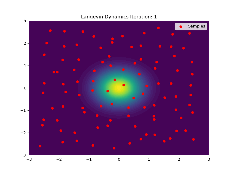
MAP Estimation with General Gaussian
Revisiting the MAP estimation problem, we can consider a more general prior \(\pi(x)\) with mean \(\mu = 0\) and covariance \(\Sigma\):
\[ \begin{align*} \pi(b|x) &= \frac{1}{(2\pi \sigma^2)^{m/2}} \exp\left(-\frac{1}{2\sigma^2}\|b-F(x)\|^2 \right)\\ \pi_\theta(x) &= \frac{1}{(2\pi)^{n/2}|\Sigma|^{1/2}} \exp\left(-\frac{1}{2}x^\intercal \Sigma^{-1} x\right)\\ \text{MAP} &= \min_x \left( \frac{1}{2\sigma^2}\|b-F(x)\|^2 + \frac{1}{2}x^\intercal \Sigma^{-1} x \right) \end{align*} \]
We now make a choice of which \(\pi_\theta(x)\) to use; as before, this is an MLE based on the available empirical samples. For the purpose of finding the gradient, let the minimization parameter be \(\theta = \Sigma^{-1}\); since the true \(\Sigma\) is positive definite, it can be recovered by inverting the result. The partition function \(Z(\theta)\) is known for the case of a Gaussian distribution, so the MLE objective is:
\[ \begin{align*} \hat\theta &= \argmax_\theta \prod_{i=1}^N \pi_\theta(x_i)\\ &= \argmax_\theta \frac{1}{Z(\theta)^N} \exp\left(-\sum_{i=1}^N \frac{1}{2}x_i^\intercal \Sigma^{-1} x_i\right)\\ &= \operatorname*{argmin}_\theta N \log(Z(\theta)) + \frac{1}{2} \sum_{i=1}^N x_i^\intercal \Sigma^{-1} x_i\\ &= \operatorname*{argmin}_\theta \log\left((2\pi)^{n/2}|\Sigma|^{1/2}\right) + \frac{1}{2N} \sum_{i=1}^N x_i^\intercal \Sigma^{-1} x_i\\ &= \operatorname*{argmin}_\theta \frac{1}{2}\log(|\Sigma|) + \frac{1}{2N} \sum_{i=1}^N x_i^\intercal \Sigma^{-1} x_i \end{align*} \]
where the constant \(\frac{n}{2}\log(2\pi)\) has been dropped, as it does not affect the minimizer.
Finding the Gradient
Left Term: To find the minimum, we take the gradient of each term with respect to \(\Sigma^{-1}\). The gradient of a log determinant can be found in the Matrix Cookbook (Petersen and Pedersen 2012), formula (57): \[ \nabla_{A} \log(|A|) = (A^{-1})^\intercal \]
Writing the left term in terms of \(A = \Sigma^{-1}\), using \(\log(|\Sigma|) = -\log(|A|)\):
\[ \nabla_{\Sigma^{-1}} \left( \frac{1}{2}\log(|\Sigma|) \right) = \nabla_A \left( -\frac{1}{2}\log(|A|) \right) = -\frac{1}{2} (A^{-1})^\intercal = -\frac{1}{2} \Sigma^\intercal\]
Right Term: The gradient of the second term is found by reformulating it as a trace of a new matrix \(X = \sum x_i x_i^\intercal\):
\[ \begin{align*} \sum x_j^\intercal \Sigma^{-1} x_j &= \sum \text{trace} \left( x_j^\intercal \Sigma^{-1} x_j \right)\\ &= \sum \text{trace} \left( \Sigma^{-1} x_j x_j^\intercal \right)\\ &= \text{trace} \left( \Sigma^{-1} X\right)\\ \end{align*} \]
The matrix cookbook (Petersen and Pedersen 2012) formula (100) gives the gradient of the trace of a matrix product:
\[ \nabla_X \text{trace}(XB) = B^\intercal\]
Applying this we get:
\[ \nabla_{\Sigma^{-1}} \left( \frac{1}{2N} \sum x_i^\intercal \Sigma^{-1} x_i \right) = \frac{1}{2N} X^\intercal = \frac{1}{2N} \sum x_i x_i^\intercal\]
Combined Result:
Combining the two terms, we get the gradient of the MLE objective with respect to \(\Sigma^{-1}\): \[ \begin{align*} g &= \nabla_{\Sigma^{-1}} \left( \frac{1}{2}\log(|\Sigma|) + \frac{1}{2N} \sum_{i=1}^N x_i^\intercal \Sigma^{-1} x_i \right)\\ &= -\frac{1}{2} \Sigma^\intercal + \frac{1}{2N} \sum_{i=1}^N x_i x_i^\intercal \end{align*} \]
Solving for where the gradient is zero, and using the symmetry \(\Sigma = \Sigma^\intercal\), we find the optimal value of \(\Sigma\):
\[ \Sigma = \frac{1}{N} \sum_{i=1}^N x_i x_i^\intercal\]
This is the maximum likelihood estimate of the covariance matrix \(\Sigma\) given the samples \(\{x_1, x_2, ..., x_N\}\), which can be interpreted as the empirical expectation of the outer product of the samples — that is, the sample covariance of the data. This is a common pattern in statistics, analogous to the sample mean being the MLE of the true mean of a distribution.
Unfortunately, estimating parameters can be very difficult for non-Gaussian \(\pi_\theta\) due to the partition function \(Z(\theta)\) being intractable.
Conclusion
MAP estimation on an inverse problem may require the use of a prior distribution \(\pi(x)\) to regularize the solution. The potential function \(\phi(x, \theta)\) is used to define the probability distribution \(\pi(x; \theta)\), and the score function \(s(x, \theta)\) is the negative gradient of the potential function.
If the prior is not known, an MLE estimate can be made to find the parameters \(\theta\) that maximize the likelihood of the samples based on an assumed parameterized model. The score matching gradient is used to estimate the gradient of the MLE objective with respect to \(\theta\).