Tikhonov regularization is a common technique used in inverse theory to stabilize ill-posed problems. In this lecture, we derive the Tikhonov regularization technique, we also have a look at a least squares solution that does not require the computation of the full SVD of the matrix \(A\), using the conjugate gradient method.
Author
Simon Ghyselincks
Published
September 20, 2024
$$
$$
Tikhnov Regularization
We have looked at the least squares formulation for solving inverse problems:
\[ \min \frac{1}{2} \|A x - b\|^2 \]
where \(A \in \mathbb R^{m \times n}\) is a linear operator, \(x \in \mathbb R^n\) is the unknown model, and \(b \in \mathbb R^m\) is the data.
The least squares problem is often ill-posed, meaning that the solution is not unique or stable. If there are more unknowns than equations, such as the case when \(n > m\), then the problem is underdetermined and there are infinitely many solutions.
We can return to unique solutions by adding a regularization term to the selection of the \(x\) that we want to minimize. The Tikhonov regularization technique adds a penalty term to the least squares problem:
where \(L \in \mathbb R^{n \times n}\) is a regularization matrix. The regularization matrix \(L\) is often chosen to be the identity matrix, but other choices are possible.
Uniqueness
To check the uniqueness of the solution, we can rewrite the problem as a quadratic form:
\[ \min \frac{1}{2} x^T A^T A x - b^T A x + \frac{1}{2} \lambda x^T L^T L x \]\[ = \min \frac{1}{2} x^T H x - b^T A x + \frac{1}{2}\|b\|^2\]
where \(H = A^T A + \lambda L^T L\) is the Hessian matrix which is symmetric and positive semi-definite by spectral theorem. If we choose an appropriate \(\lambda\), then the Hessian matrix is positive definite and the problem is well-posed. In the case where \(L=I\), the Hessian becomes full rank for \(\lambda > 0\) and the problem is well-posed. The quality that \(H \succ 0\) means that the matrix is invertible.
Solution
The unique solution is given by by the first order optimatility condition:
\[ \begin{align}
(A^T A + \lambda L^T L) \mathbf{x}_{\text{RLS}} - A^T b&= 0 \\
\mathbf{x}_{\text{RLS}} &= (A^T A + \lambda L^T L)^{-1} A^T b
\end{align}
\]
SVD Decomposition
The solution can be written in terms of the singular value decomposition of \(A\), and with the assumption that \(L=I\):
\[ \begin{align}
A &= U \Sigma V^T \\
A^T A &= V \Sigma^T \Sigma V^T \\
\mathbf{x}_{\text{RLS}} &= \left( V \Sigma^2 V^T + \lambda I \right)^{-1} V \Sigma^T U^T b \\
&= \left( V \Sigma^2 V^T + \lambda I V V^T \right)^{-1} V \Sigma^T U^T b\\
&= V \left( \Sigma^2 + \lambda I \right)^{-1} \Sigma^T U^T b\\
&= V \mathbf{Diag}\left( \frac{\sigma_i}{\sigma_i^2 + \lambda} \right) U^T b\\
&= \sum _i ^ n \frac{\sigma_i}{\sigma_i^2 + \lambda} \langle u_i, b \rangle v_i
\end{align}
\]
This form is more readily comparable to some of the other methods that we have see so far, which are presented in the table below:
Comparison of Least Squares Methods
Method
Solution
Tikhonov
\(x_{\text{RLS}} = \sum _i ^ n \frac{\sigma_i}{\sigma_i^2 + \lambda} \langle u_i, b \rangle v_i\)
Thresholded SVD
\(x_{\text{TSVD}} = \sum _i ^ n h(\sigma_i) \langle u_i, b \rangle v_i\)
Gradient Flow
\(x_{\text{SDF}} = \sum _i ^ n \frac{\exp(-\sigma_i^2 t) - 1}{\sigma_i} \langle u_i, b \rangle v_i\)
As we can see all three methods have a similar form and offer some mechanism for controlling the noise induced by the small singular values of \(A\).
Show the code
import numpy as npimport matplotlib.pyplot as pltimport seaborn as snsdef generate_ill_conditioned_matrix(m, n, condition_number): # Generate random orthogonal matrices U and V U, _ = np.linalg.qr(np.random.randn(m, m)) V, _ = np.linalg.qr(np.random.randn(n, n)) sigma = np.linspace(1, 1/condition_number, min(m, n)) Sigma = np.diag(sigma) A = U @ Sigma @ V[:min(m, n), :]return A, sigma# Seed for reproducibilitynp.random.seed(4)A, S = generate_ill_conditioned_matrix(8, 24, 1e3)# Create a vector b of size 5 with random valuesb = np.random.randn(8)# Compute the SVD of AU, S, Vt = np.linalg.svd(A, full_matrices=False)V = Vt.TU = U # Already in proper shape# Number of singular valuesn =len(S)# Define parameters for each method# Gradient Flowt_values = np.linspace(0, 0.6, 100)# Tikhonov Regularizationlambda_values = np.linspace(1e-4, 1, 100)# Thresholded SVDthreshold_values = np.linspace(0, max(S), 100)# Compute scaling factors for each method# Gradient Flow Scaling
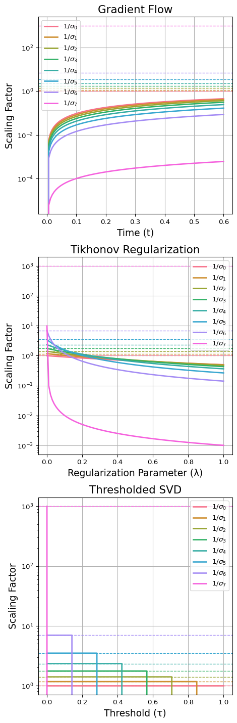
def gradient_flow_scaling(sigma, t):return (1- np.exp(-sigma**2* t)) / sigmagradient_scalings = np.array([gradient_flow_scaling(s, t_values) for s in S])# Tikhonov Scalingdef tikhonov_scaling(sigma, lambd):return sigma / (sigma**2+ lambd)tikhonov_scalings = np.array([tikhonov_scaling(s, lambda_values) for s in S])# Thresholded SVD Scalingdef tsvd_scaling(sigma, threshold):return np.where(sigma >= threshold, 1/sigma, 0)tsvd_scalings = np.array([tsvd_scaling(s, threshold_values) for s in S])# Initialize the plot with 3 subplotsfig, axes = plt.subplots(3, 1, figsize=(5, 15))# Define a color palettepalette = sns.color_palette("husl", n)# Plot Gradient Flowax = axes[0]for i inrange(n): ax.plot(t_values, gradient_scalings[i], color=palette[i], linewidth=2, label=f'$1/\sigma_{i}$' ) ax.axhline(y=1/S[i], color=palette[i], linestyle='--', linewidth=1)ax.set_yscale('log')ax.set_xlabel('Time (t)', fontsize=14)ax.set_ylabel('Scaling Factor', fontsize=14)ax.set_title('Gradient Flow', fontsize=16)ax.legend()ax.grid(True)# Plot Tikhonov Regularizationax = axes[1]for i inrange(n): ax.plot(lambda_values, tikhonov_scalings[i], color=palette[i], linewidth=2, label=f'$1/\sigma_{i}$' ) ax.axhline(y=1/S[i], color=palette[i], linestyle='--', linewidth=1)ax.set_yscale('log')ax.set_xlabel('Regularization Parameter (λ)', fontsize=14)ax.set_ylabel('Scaling Factor', fontsize=14)ax.set_title('Tikhonov Regularization', fontsize=16)ax.legend()ax.grid(True)# Plot Thresholded SVDax = axes[2]for i inrange(n): ax.plot(threshold_values, tsvd_scalings[i], color=palette[i], linewidth=2, label=f'$1/\sigma_{i}$') ax.axhline(y=1/S[i], color=palette[i], linestyle='--', linewidth=1)ax.set_yscale('log')ax.set_xlabel('Threshold (τ)', fontsize=14)ax.set_ylabel('Scaling Factor', fontsize=14)ax.set_title('Thresholded SVD', fontsize=16)ax.legend()ax.grid(True)# Adjust layout and add a legendplt.tight_layout()plt.show()
Evolution of scaling factors for three different methods
Solving Least Squares Using Conjugate Gradient
A detailed explanation of this method can be found at Wikipedia
Conjugate Vectors Definition
A set of vectors \(\{ p_1, p_2, \ldots, p_n \}\) is said to be conjugate with respect to a matrix \(A\) if:
\[
\langle p_i, A p_j \rangle = 0 \quad \text{for all } i \neq j
\]
This is a generalization of the concept of orthoganality to non-symmetric matrices.
Standard Orthogonality: When $ A = I $ (the identity matrix), the definition reduces to the standard concept of orthogonality. For a symmetric \(A\) we also have an orthogonal decomposition of eigenvectors by spectral theorem.
Back to the problem of least squares, we can express the solution $ x $ as a linear combination of conjugate vectors:
\[
x = x_0 + \sum_{i=1}^n \alpha_i p_i
\]
where:
\(x_0\) is an initial guess (can be zero).
\(\alpha_i\) are scalar coefficients.
\(p_i\) are conjugate vectors with respect to \(A\).
To recover the coefficients of \(\alpha_i\) we can use a projection in the weighted space of \(A\):
\[ \begin{align}
A x_0 + \sum_{i=1}^n \alpha_i A p_i &= b\\
r &= b - A x_0\\
\sum_{i=1}^n \alpha_i A p_i &= r\\
\langle p_i, \sum_{i=1}^n \alpha_i A p_i \rangle &= \langle p_i, r \rangle\\
\alpha_i \langle p_i, A p_i \rangle &= \langle p_i, r \rangle\\
\alpha_i &= \frac{\langle p_i, r \rangle}{\langle p_i, A p_i \rangle}
\end{align}
\] In the case where \(x_0\) is zero, then this reduces to \[ \alpha_i = \frac{\langle p_i, b \rangle}{\langle p_i, A p_i \rangle} \]
The method can be seen better if we trace through the minimization problem for fixed \(x\) and with variable \(\alpha\):
\[
\begin{align}
& \min \frac{1}{2} \|A (x+\alpha p) - b\|^2 \\
&= \frac{1}{2}r^T r + \alpha \langle r, A p \rangle + \frac{1}{2} \alpha^2 \langle p, A^T A p \rangle \\
0 &= \langle r, A p \rangle + \alpha \langle p, A^T A p \rangle \\
\alpha &= -\frac{\langle r, A p \rangle}{\|A p\|^2}
\end{align}
\]
But we can also trace this through using the expansion of lest squares and removing the \(\|b\|^2\) term:
\[
\begin{align}
& \min \frac{1}{2} \tilde x^T A x - \tilde x^T b \\
&= \frac{1}{2} \left( x^T A x + 2 \alpha x^T A p + \alpha^2 p^T A p \right) - x^T b - \alpha p^T b\\
0&= x^TAp + \alpha p^T A p - p^T b \\
\alpha &= \frac{p^T (Ax-b)}{p^T A p}
\end {align}
\]