Lecture 5

Gauss Newton for Non-Linear Least Squares Optimization

The Gauss-Newton method is a powerful optimization technique for solving non-linear least squares problems of the form \(\min_{p} \frac{1}{2}\|F(p)-d\|^2\). In this lecture, a derivation of the method is presented along with a comparison to Newton’s method. Finally an algorithm for solving the problem is given.

$$

$$

A Non-Linear Dynamics Problem

A well studied problem in non-linear dynamics involves the predator-prey model that is described by the Lotka-Volterra equations. The equations are given by:

\[ \begin{aligned} \frac{dx}{dt} &= \alpha x - \beta xy \\ \frac{dy}{dt} &= \delta xy - \gamma y \end{aligned} \]

where \(x\) and \(y\) are the populations of the prey and predator respectively. The parameters \(\alpha, \beta, \gamma, \delta\) are positive constants. The goal is to find the values of these parameters that best fit the data.

No closed-form analytic solution is known for this remarkably simple system of equations, which is why we must resort to numerical methods to compute the model.

More information about the model can be found on the Wikipedia page.

The Forward Problem

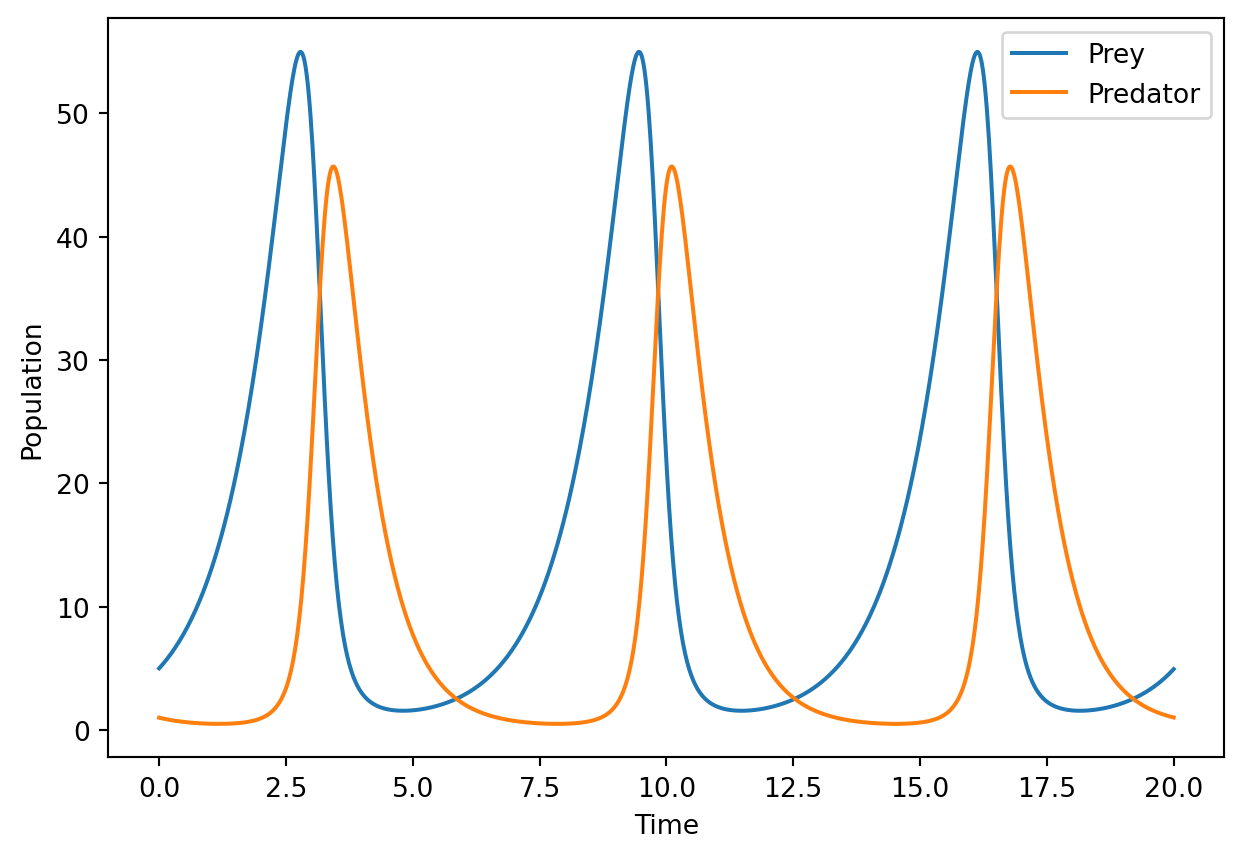
We start with an initial time \(t_0\) and initial conditions \(x_0, y_0\), along with parameters \(\alpha, \beta, \gamma, \delta\), and run the forward problem using the classical fourth-order Runge-Kutta method (RK4), a higher-order relative of the forward Euler method.

import numpy as np
import matplotlib.pyplot as plt
import torch
import torch.nn as nn

class LotkaVolterraModel(nn.Module):
    def __init__(self, alpha, beta, gamma, delta):
        super(LotkaVolterraModel, self).__init__()
        # Define parameters as torch tensors that require gradients
        self.alpha = nn.Parameter(torch.tensor(alpha, dtype=torch.float32))
        self.beta = nn.Parameter(torch.tensor(beta, dtype=torch.float32))
        self.gamma = nn.Parameter(torch.tensor(gamma, dtype=torch.float32))
        self.delta = nn.Parameter(torch.tensor(delta, dtype=torch.float32))

    def forward(self, x, y):
        # Ensure x and y are tensors
        if not isinstance(x, torch.Tensor):
            x = torch.tensor(x, dtype=torch.float32)
        if not isinstance(y, torch.Tensor):
            y = torch.tensor(y, dtype=torch.float32)

        # Compute dx and dy based on the current parameters
        dx = self.alpha * x - self.beta * x * y
        dy = self.delta * x * y - self.gamma * y

        return dx, dy

class RK4Solver:
    def __init__(self, model):
        self.model = model

    def step(self, x, y, dt):
        """
        Perform a single RK4 step.
        """
        # Convert x and y to tensors if they are not already
        if not isinstance(x, torch.Tensor):
            x = torch.tensor(x, dtype=torch.float32)
        if not isinstance(y, torch.Tensor):
            y = torch.tensor(y, dtype=torch.float32)

        # RK4 Step calculations
        k1_x, k1_y = self.model.forward(x, y)
        k2_x, k2_y = self.model.forward(x + 0.5 * dt * k1_x, y + 0.5 * dt * k1_y)
        k3_x, k3_y = self.model.forward(x + 0.5 * dt * k2_x, y + 0.5 * dt * k2_y)
        k4_x, k4_y = self.model.forward(x + dt * k3_x, y + dt * k3_y)

        # Update x and y using weighted averages of the slopes
        x_new = x + (dt / 6) * (k1_x + 2 * k2_x + 2 * k3_x + k4_x)
        y_new = y + (dt / 6) * (k1_y + 2 * k2_y + 2 * k3_y + k4_y)

        return x_new, y_new

    def solve(self, x0, y0, time_steps):
        """
        Solve the system over a series of time steps.
        Parameters:
            x0: Initial value of prey population
            y0: Initial value of predator population
            time_steps: List or numpy array of time steps to solve over
        """
        x, y = x0, y0
        DT = time_steps[1:] - time_steps[:-1]
        trajectory = torch.zeros(len(time_steps), 2)
        trajectory[0] = torch.tensor([x, y])

        for i, dt in enumerate(DT):
            x, y = self.step(x, y, dt)
            trajectory[i+1] = torch.tensor([x, y])            

        return trajectory

# Define the model parameters
alpha = 1.0
beta = .1
gamma = 1.5
delta = 0.1

# Create the model and solver
model = LotkaVolterraModel(alpha, beta, gamma, delta)
solver = RK4Solver(model)

# Define the initial conditions and time steps
x0 = 5
y0 = 1
time_steps = np.linspace(0, 20, 1000)

# Solve the system
trajectory = solver.solve(x0, y0, time_steps)

x_values = trajectory[:, 0].detach().numpy()
y_values = trajectory[:, 1].detach().numpy()

plt.plot(time_steps, x_values, label='Prey')
plt.plot(time_steps, y_values, label='Predator')
plt.xlabel('Time')
plt.ylabel('Population')
plt.legend()
plt.savefig('imgs/lotka_volterra.png')
plt.show()

The time evolution of the prey and predator populations.

We can additionally look at the phase space of the system for various initial conditions to see how the different solutions are periodic.

# Define the initial conditions
x0 = 5
y0 = [.2,.5,1, 2, 3, 4, 5]

# Create the model and solver
model = LotkaVolterraModel(alpha, beta, gamma, delta)
solver = RK4Solver(model)

# Define the time steps
time_steps = np.linspace(0, 10, 1000)

# Plot the phase space
plt.figure(figsize=(6, 4.5))
for y in y0:
    trajectory = solver.solve(x0, y, time_steps)
    x_values = trajectory[:, 0].detach().numpy()
    y_values = trajectory[:, 1].detach().numpy()
    plt.plot(x_values, y_values, label=f'y0={y}')

plt.xlabel('Prey Population')
plt.ylabel('Predator Population')
plt.legend()
plt.title('Lotka-Volterra Phase Space')
plt.savefig('imgs/lotka_volterra_phase_space.png')
plt.show()

The phase space of the predator-prey model.

The Inverse Problem

The inverse problem in this case is to find the parameters \(\alpha, \beta, \gamma, \delta\) that best fit the data. We suppose that we have a parameterized model that takes in the initial conditions and time steps and returns the trajectory of the system. For simplicity we vectorize the previous \(\begin{bmatrix} x \\ y \end{bmatrix}\) into a single state vector \(\vec{x}\). The system dynamics are then described by a function \(f(\vec{x}; \vec{p})\), where \(\vec{x}\) is the state of the system and \(\vec{p}\) are the parameters:

\[f(\vec{x}; \vec{p}) \approx \frac{d \vec{x}}{dt} = \begin{bmatrix} \alpha x - \beta xy \\ \delta xy - \gamma y \end{bmatrix}, \quad \vec{x}_0 = \vec{x}(0).\]

The goal is to form an estimate of \(\vec{p}\), while the data that we have collected may be sparse, noisy, or incomplete. We represent the incompleteness of the data using a sampling operator \(Q\), which is applied to the true underlying data to give \(Qx\). If \(x\) is fully observed, then \(Q = I\).

A finite difference approximation can be used to estimate the time derivative of the data,

\[f(\vec{x}; \vec{p}) \cong \frac{\vec{x}_{n+1} - \vec{x}_n}{\Delta t}.\]

The forward process applies the system dynamics to the initial condition \(\vec{x}_0\) using an approximate ODE solver such as Euler’s method or RK4. The output of the forward process is then given as \(F\), where \[F(\vec{p}, x_0) = \hat {\vec{x}}(t, \vec{p})\]

is the estimated trajectory produced by applying the system dynamics to the initial conditions and parameters.

The observed data is \(d = Q\vec{x}(t)\). We also assume that \(F\) does not depend on the particular solver used for the forward ODE, and that all of the \(\vec{p}\) are physical parameters — that is, the parameterization is faithful enough to the true system.

For the rest of the mathematical notation ahead, the explicit marking of vectors is omitted to simplify the equations.

Goodness of Fit

The goodness of fit is measured using the L2 norm of the difference between the observed data and the model output, thus forming the non-linear least squares problem:

\[ \min_{p} \frac{1}{2}\|QF(p)-d\|^2 = \min_{p} \frac{1}{2}\|G(p)\|^2.\]

To find the best fit, the objective is to minimize this squared misfit between the model output and the data \(d\). The data is fixed for a given problem, so it is only by varying \(p\) that an optimal solution can be found. The residual function is denoted \(G(p) = QF(p) - d\).

Minimization of the Objective Function

\[ \min_{p \in \mathbb{R}^m} \biggl\{ \sum_{i=1}^n (QF_i(\mathbf{p}) - d_i) ^2\biggr\}\]

where \(d_i\) are the observed data points. This is the same as

\[ \min_{p \in \mathbb{R}^m} \|G(\mathbf{p})\|^2\]

where \(G(\mathbf{p}) = QF(\mathbf{p}) - d\) and \(d \in \mathbb{R}^n\). We are minimizing the norm of a non-linear function of the parameters. Supposing that we want to find the minimizer, one approach would be gradient descent.

The Jacobian: A quick review

---

The Jacobian is a multivariate extension of the derivative that applies to functions \(f : \mathbb{R}^m \to \mathbb{R}^n\). Because there are \(n\) function outputs and \(m\) input variables, the Jacobian is an \(n \times m\) matrix that captures how each of the \(n\) outputs changes with respect to each of the \(m\) variables. In an abuse of Leibniz’s notation, it can be seen as:

\[ \frac{\partial \vec{f}}{\partial \vec{x}} = \mathbf{J_f} = \left[ \frac{\partial f}{\partial x_1} \cdots \frac{\partial f}{\partial x_m} \right] = \begin{bmatrix} \nabla^\top f_1 \\ \vdots \\ \nabla^\top f_n \end{bmatrix} = \left[ \begin{array}{ccc} \frac{\partial f_1}{\partial x_1} & \cdots & \frac{\partial f_1}{\partial x_m} \\ \vdots & \ddots & \vdots \\ \frac{\partial f_n}{\partial x_1} & \cdots & \frac{\partial f_n}{\partial x_m} \end{array} \right] \]

Note that, like the derivative, the Jacobian is a function of the input variables \(\vec{x}\). The Jacobian gives a linear approximation of the function \(f\) at a point \(x_0\), which can be used to approximate the function at a nearby point \(x_0 + \Delta x\):

\[ f(x_0 + \Delta x) \approx f(x_0) + J_f(x_0) \Delta x\]

Note that we are applying matrix multiplication, using \(J_f\) evaluated at \(x_0\) and the vector \(\Delta x = \vec{x} - \vec{x_0}\). The quantity \(J_f(x_0) \Delta x\) is the directional derivative of the function \(f\) at \(x_0\) in the direction of \(\Delta x\).

---

The gradient of \(\|G(\mathbf{p})\|^2\) can be computed as follows:

\[\begin{align} \nabla_p \|G(p)\|^2 &= \nabla_p G(p)^T G(p)\\ &= \sum_{i=1}^n \nabla_p G_i(p)^2\\ &= \sum_{i=1}^n 2 G_i(p) \nabla_p G_i(p)\\ &= 2 J_G(p)^T G(p) \end{align} \]

From this stage, gradient descent can be applied to find the minimum of the function. However, the function \(G(p)\) is non-linear and so the gradient descent method may not converge quickly or the problem may have poor conditioning. The celebrated Newton’s Method addresses some of these issues, but requires computing the Hessian \(\nabla^2 \|G(p)\|^2\) of the function, which can be expensive.

To demonstrate, the true Hessian of the function is: \[ \nabla^2 \|G(p)\|^2 = 2 J_G(p)^T J_G(p) + 2 \sum_{i=1}^n G_i(p) \nabla^2 G_i(p) \]

So we would have to compute the Hessian \(\nabla^2 G_i(p)\) of each of the \(G_i(p)\) functions, of which there are \(n\) — impractical for problems of any real size. If we did have this Hessian, the steps with Newton’s method would be:

\[ p_{k+1} = p_k - (\nabla^2 \|G(p_k)\|^2)^{-1} \nabla (\|G(p_k)\|^2)\]

Gauss-Newton Optimization

Rather than solve the problem directly with Newton’s method, it can be approximated by linearizing inside of the norm and solving the linearized version using the normal equations. We approximate the function

\[G(p) = QF(p) - d \approx (QF(p_k) - d) + QJ_k(p-p_k)\]

where \(J_k\) is the Jacobian of \(F(p)\) at \(p_k\).

\[ \min_{p \in \mathbb{R}^m} \|QF(p_k) - d + QJ_k(p-p_k)\|^2\]

Then rearranging this we get a form that is a linear least squares problem:

\[ \begin{align} & \min_{p \in \mathbb{R}^m} \| QJ_kp - (d + QJ_k p_k- QF(p_k) )\|^2\\ =& \min_{p \in \mathbb{R}^m} \| Ap - r_k\|^2\\ A^T A p =& A^T r_k \end{align} \]

where \(A = QJ_k\) and \(r_k = d + QJ_k p_k - QF(p_k)\). These are the normal equations for the linear least squares problem. This gives us

\[ \begin{align} p_{k+1} &= (A^T A)^{-1} A^T (r_k)\\ &= (J_k^T Q^T Q J_k)^{-1} J_k^T Q^T (d + QJ_k p_k - QF(p_k))\\ &= p_k + (J_k^T Q^T Q J_k)^{-1} J_k^T Q^T (d - QF(p_k))\\ p_{k+1} &= p_k - (J_k^T Q^T Q J_k)^{-1} J_k^T Q^T (QF(p_k) - d)\\ \end{align} \]

This can be written in a tidier and more general way: recalling that \(G(p) = QF(p) - d\) and letting \(J_G(p) = QJ(p)\), we have:

\[ p_{k+1} = p_k - (J_G(p_k)^TJ_G(p_k))^{-1} J_G(p_k)^T G(p_k)\]

Comparison with Newton’s Method

So this resembles a scaled gradient descent. In Newton’s method the scaling is the full Hessian; in Gauss-Newton it is built from the Jacobian of the residual function. As a comparison:

Method	Step Update	Scaling Matrix
Newton’s Method	\(p_{k+1} = p_k - (\nabla^2 \|G(p_k)\|^2)^{-1} \nabla \|G(p_k)\|^2\)	\(\nabla^2 \|G(p_k)\|^2 = 2 J_G(p_k)^T J_G(p_k) + 2 \sum_{i=1}^n G_i(p_k) \nabla^2 G_i(p_k)\)
Gauss-Newton Method	\(p_{k+1} = p_k - (J_G(p_k)^T J_G(p_k))^{-1} J_G(p_k)^T G(p_k)\)	\(J_G(p_k)^T J_G(p_k)\)

The direction of change between iterations in Newton’s method can be rewritten as \[d_k = \left(J_G(p_k)^T J_G(p_k) + \sum_{i=1}^n G_i(p_k) \nabla^2 G_i(p_k)\right)^{-1} J_G(p_k)^T G(p_k)\]

while the direction in the case of Gauss-Newton is \[d_k = \left(J_G(p_k)^T J_G(p_k)\right)^{-1} J_G(p_k)^T G(p_k)\]

The difference between the two is the omission of the computationally expensive \(\sum_{i=1}^n G_i(p) \nabla^2 G_i(p)\) terms. The Gauss-Newton method approximates the second-order approach of Newton’s method by considering only the first-order terms inside of the norm:

\[J_G(p_k)^T J_G(p_k) + \sum_{i=1}^n G_i(p_k) \nabla^2 G_i(p_k) \approx J_G(p_k)^T J_G(p_k)\]

Recall that \(G(p) = QF(p) - d\) which is the difference between the observed data and the model. If the difference is small then \(G_i\) is also small and the approximation is good.

Algorithm for Gauss-Newton

We have derived the algorithm for the Gauss-Newton method for solving the non-linear least squares problem. The algorithm is as follows:

\begin{algorithm} \caption{Gauss-Newton Algorithm for Non-linear Least Squares}\begin{algorithmic} \State \textbf{Input:} Initial guess $p_0$, maximum iterations $K$, tolerance $\epsilon$ \State \textbf{Initialize} $p_0$ \For{$k = 0, 1, 2, \ldots$} \State Compute the Jacobian $J_G$ of $G(p)$ at $p_k$ \State Compute the transpose $J_G^T$ of the Jacobian \State Compute the residual $r_k = -G(p_k) = d - QF(p_k)$ (forward model) \State Compute the step $s_k = (J_G(p_k)^T J_G(p_k) )^{-1} J_G(p_k)^T r_k$ \State Update the parameters $p_{k+1} = p_k + \mu_k s_k$ \If{$\|s_k\| < \epsilon$} \State \textbf{Stop} \EndIf \EndFor \State \textbf{Output:} $p_{k+1}$ as the optimal solution \end{algorithmic} \end{algorithm}

Here \(\mu_k \in (0, 1]\) is an optional step length (damping) parameter, which can be chosen by a line search; \(\mu_k = 1\) recovers the pure Gauss-Newton step.

Matrix Inversions

In practice it may be computationally expensive to invert the matrix \(J_k^T Q^T Q J_k\). We can use a conjugate gradient method to solve the normal equations instead: \[J_k^T Q^T Q J_k s_k = J_k^T Q^T r_k\]

We developed a conjugate gradient method in the last lecture, so we can use that along with the computed values for \(J_k^T, J_k, r_k\) to solve the normal equations and get the step \(s_k\).

Summary

Component	Description	Dimensions
\(d\)	Observed data	\(\mathbb{R}^{n}\)
\(p_k\)	Parameters	\(\mathbb{R}^{m}\)
\(Q\)	Sampling/weighting operator	\(\mathbb{R}^{n \times n}\)
\(J_k\)	Jacobian of \(F(p_k)\)	\(\mathbb{R}^{n \times m}\)
\(r_k\)	Residual \(d - QF(p_k)\)	\(\mathbb{R}^{n}\)
\(F(p_k)\)	Forward model output	\(\mathbb{R}^{n}\)
\(s_k\)	Step direction	\(\mathbb{R}^{m}\)
\(J_k^T\)	Transpose of the Jacobian	\(\mathbb{R}^{m \times n}\)
\(J_k^T Q^T Q J_k\)	Normal equations matrix	\(\mathbb{R}^{m \times m}\)