import numpy as np
from matplotlib.collections import LineCollection
from torch.nn.functional import pad
def generate_data_set(
initial_pop=initial_pop, period=40.0, n_time_steps=2000, n_realizations=10
):
pop_data_runs = []
perturbations = []
for run_idx in range(n_realizations):
print(f"Computing realization {run_idx + 1}/{n_realizations}")
# Generate noise for perturbing alpha across time steps
noise = torch.randn(
1, n_time_steps
) # Shape [1, n_time_steps] for a single parameter over time
for _ in range(250): # Smooth out the noise to resemble realistic fluctuations
noise = pad(noise, pad=(1, 1), mode="reflect")
noise = (noise[:, :-2] + 2 * noise[:, 1:-1] + noise[:, 2:]) / 4
noise = noise.squeeze() # Shape [n_time_steps]
# Base parameters without perturbation, as shape [n_time_steps, 4]
base_params = torch.tensor([4 / 3, 2 / 3, 1, 1]).expand(n_time_steps, 4)
# Apply perturbation to alpha (the first parameter)
params = base_params.clone()
params[:, 0] += noise # Modify alpha over time
# Solve ODE with perturbed parameters
pop_data = lotka_volterra(params, initial_pop, T=period, nt=n_time_steps)
pop_data_runs.append(pop_data)
perturbations.append(noise)
return pop_data_runs, perturbations
initial_pop = torch.rand(2)
XX, M = generate_data_set(
initial_pop=initial_pop, period=period, n_time_steps=n_time_steps, n_realizations=1
)
X = XX[0]
pert = M[0]
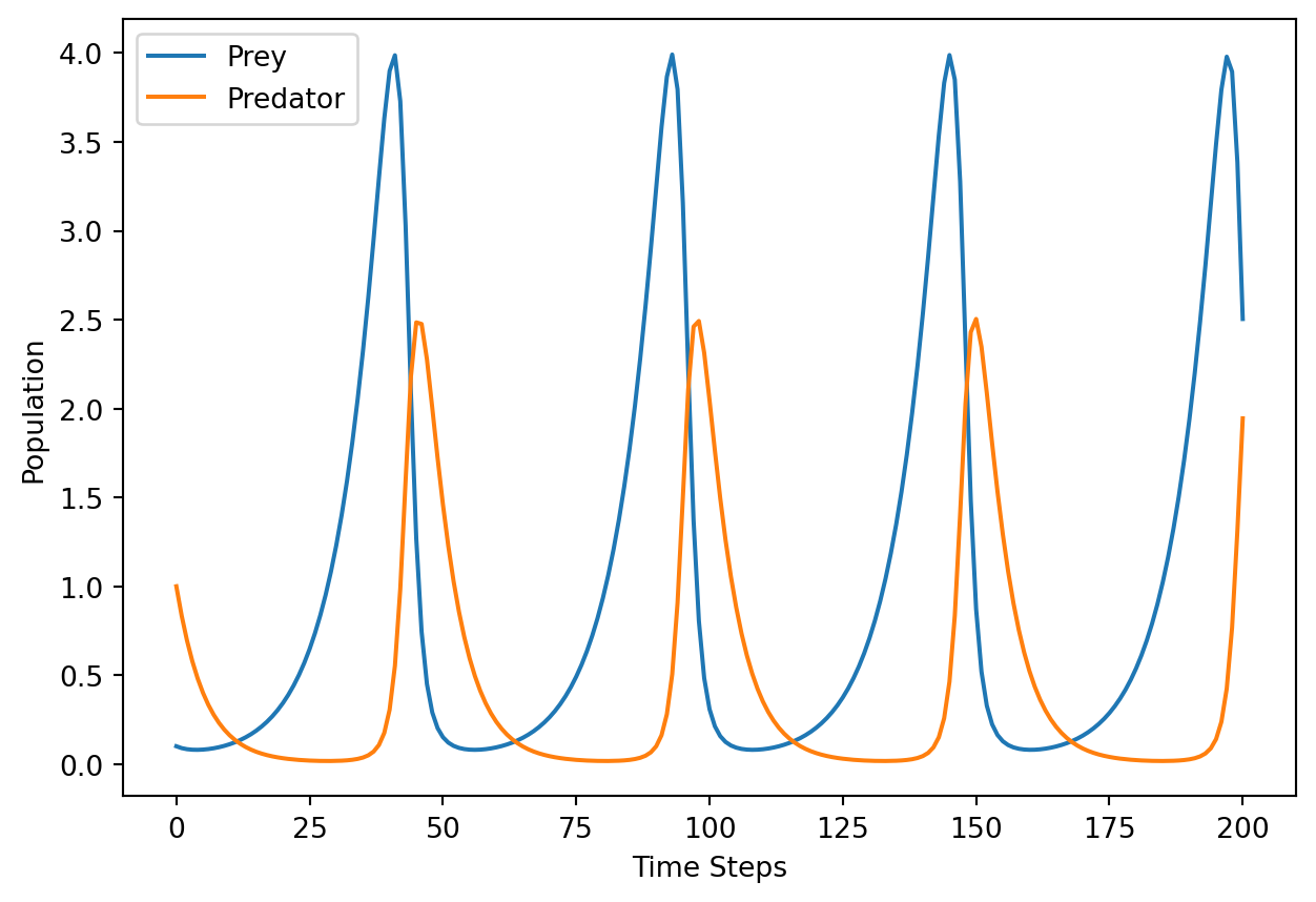
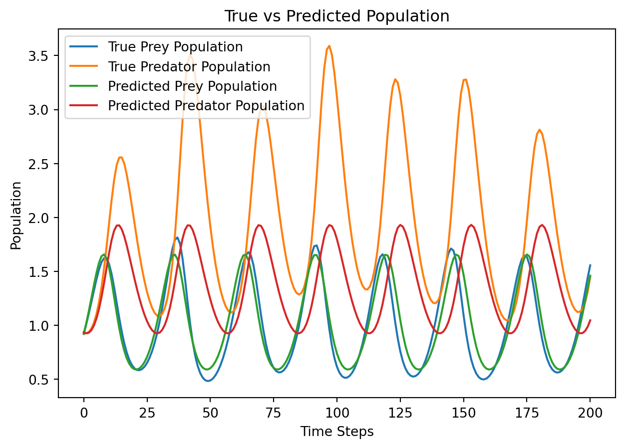
d_true = X[0, :] # Use the prey population as the data to fit
# Time series plot
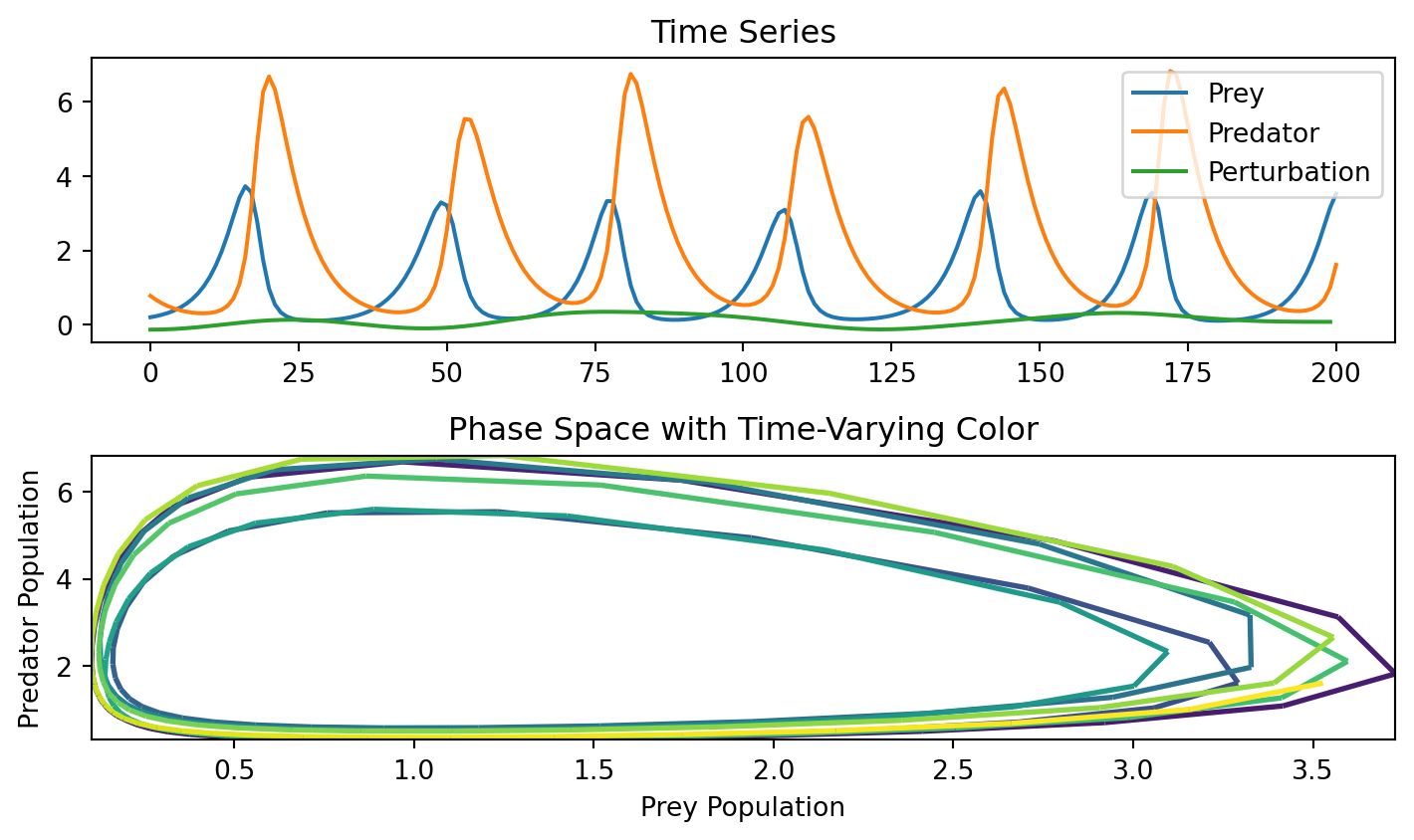
plt.figure(figsize=(7.5, 4.5))
plt.subplot(2, 1, 1)
plt.plot(X[0, :].detach(), label="Prey")
plt.plot(X[1, :].detach(), label="Predator")
plt.plot(pert.detach(), label="Perturbation")
plt.legend()
plt.title("Time Series")
# Phase space plot with color gradient
plt.subplot(2, 1, 2)
# Prepare data for LineCollection
prey = X[0, :].detach().numpy()
predator = X[1, :].detach().numpy()
points = np.array([prey, predator]).T.reshape(-1, 1, 2)
segments = np.concatenate([points[:-1], points[1:]], axis=1)
cmap = "viridis"
# Create a LineCollection with the chosen colormap
lc = LineCollection(segments, cmap=cmap, norm=plt.Normalize(0, 1))
lc.set_array(np.linspace(0, 1, len(segments))) # Normalize color range to [0,1]
lc.set_linewidth(2)
# Add the LineCollection to the plot
plt.gca().add_collection(lc)
# Set plot limits to the data range
plt.xlim(prey.min(), prey.max())
plt.ylim(predator.min(), predator.max())
plt.title("Phase Space with Time-Varying Color")
plt.xlabel("Prey Population")
plt.ylabel("Predator Population")
plt.tight_layout()
plt.show()