import numpy as np
import matplotlib.pyplot as plt
from scipy.fft import dct, idct
import time

def hutchinson(A, num_queries, dist="rademacher"):
    n = A.shape[0]
    if dist == "rademacher":
        V = np.random.randint(0, 2, size=(n, num_queries)) * 2 - 1
    elif dist == "gaussian":
        V = np.random.randn(n, num_queries)

    Y = A @ V
    trace_est = np.sum(V * Y) / num_queries
return trace_estTrace Estimation for Implicit Matrices
A Hutchinson’s and Hutch++ Survey
Randomized Algorithms
Linear Algebra
Machine Learning
Implicit matrix trace estimation using only matrix-vector products is a problem that commonly arises in many areas of scientific computing and machine learning. This work explores randomized algorithms including Hutchinson’s and Hutch++.
\[ \newcommand{\mA}{\mathbf{A}} \newcommand{\mI}{\mathbf{I}} \newcommand{\mH}{\mathbf{H}} \newcommand{\mD}{\mathbf{D}} \newcommand{\mF}{\mathbf{F}} \newcommand{\mQ}{\mathbf{Q}} \newcommand{\mS}{\mathbf{S}} \newcommand{\mG}{\mathbf{G}} \newcommand{\mU}{\mathbf{U}} \newcommand{\mV}{\mathbf{V}} \newcommand{\mY}{\mathbf{Y}} \newcommand{\vv}{\mathbf{v}} \newcommand{\vz}{\mathbf{z}} \newcommand{\vw}{\mathbf{w}} \newcommand{\va}{\mathbf{a}} \newcommand{\ve}{\mathbf{e}} \newcommand{\tr}{\operatorname{Tr}} \newcommand{\Var}{\operatorname{Var}} \newcommand{\Pr}{\mathbb{P}} \]
NoteAbstract
Implicit matrix trace estimation using only matrix-vector products is a problem that commonly arises in many areas of scientific computing and machine learning. When the matrix is only accessible through matrix-vector products \(\mA \vv\) or is excessively large, classical deterministic methods for computing the trace are infeasible. This work presents a survey and comparative analysis of randomized algorithms for trace estimation, building from the foundational Hutchinson’s estimator to modern variance-reduced techniques like Hutch++. We synthesize the evolution of theoretical guarantees, moving from initial variance-based analysis to rigorous \((\epsilon, \delta)\)-concentration bounds. Furthermore, we evaluate the practical performance of these methods through numerical experiments on matrices with varying spectral properties. We empirically verify the optimal convergence rates of Hutch++ on matrices with decaying spectra and discuss the trade-offs between different probing vector distributions.
Code is available at GitHub Gist
1 Introduction
Implicit matrix trace estimation for a matrix \(\mA\) using only the matrix-vector product \(\mA \vv\) over some set of \(\mA \vv_1,\mA \vv_2,...\mA \vv_m \in \mathbb{R}^N\) is a problem that commonly arises in scientific computing and machine learning (Ubaru and Saad 2018). When \(\mA\) is only accessible through the map \(x \mapsto \mA x\), there is no direct access to its matrix elements, and we call this an implicit representation. Even in the case where \(\mA\) is explicitly computable, it may be of an excessively large dimension, making it infeasible to store and compute the full matrix. Similarly, for \(\mA \in \mathbb{R}^{N \times N}\), although \(\tr(\mA)\) is simply the sum of diagonal elements, it requires evaluating \(\sum_{i\in [N]} e_i^\top \mA e_i\), which for large \(n\) may be computationally expensive, intractable, or unnecessary for the level of precision required.
Often these problems arise within an iterative process, where an estimation will suffice under the expectation that future algorithmic steps will further refine the problem solution (Woodruff et al. 2022). This problem formulation is well suited to randomized numerical linear algebra (RNLA) techniques, and as discussed below, can even be effectively paired with other randomized algorithms such as low-rank matrix estimation for further efficiency gains (Meyer et al. 2021).
The goal of trace estimation then is to find an approximation within some error tolerance such that the total required matrix-vector products scale sublinearly in \(N\), avoiding \(O(N)\) complexity. A naive approach would be to randomly sample a subset of the diagonal elements of \(\mA\) as an estimator, but the diagonal elements may be highly concentrated, resulting in the same variance issues posed by sparse sampling (Avron and Toledo 2011). Thus we must employ more sophisticated methods to gain better approximations at a cheaper cost, as measured by both computational complexity and the total matrix-vector products. This motivates the need for generalizable methods capable of probing the structure of \(\mA\) using a limited number of matrix-vector products or other implicit representations.
1.1 Trace Estimation Applications
Examples of trace estimation problems are abundant (Ubaru and Saad 2018). In deep learning, large and complex models often require the estimation of traces of Hessian matrices \(\mH\) for optimization and uncertainty quantification. A common architecture such as ResNet-50 has a \(25 \text{ million} \times 25 \text{ million}\) matrix \(\mH\) that is prohibitive to store, but whose matrix-vector product \(\mH \vv\) can be efficiently computed using Pearlmutter’s trick (Pearlmutter 1994). High-dimensional trace estimation is also used for training Physics Informed Neural Networks (PINNs) (Hu et al. 2024). In probabilistic machine learning, trace estimation is used in score-matching methods (Song et al. 2019).
1.2 Scope of this Review
This article synthesizes the progression of Randomized Numerical Linear Algebra (RNLA) methods for trace estimation, analyzes their theoretical properties, and evaluates their performance through numerical experiments. Specifically, we:
- Review the foundational Hutchinson’s estimator (Hutchinson 1990).
- Analyze the \((\epsilon, \delta)\) bounds derived by Avron and Toledo (2011).
- Implement and verify the Hutch++ algorithm (Meyer et al. 2021), which combines low-rank approximation with stochastic estimation.
- Compare these methods numerically on matrices with different spectral decay properties.
2 Background
2.1 Notation and Definitions
In this work, lower case \(a\) denotes a scalar, capital \(A\) denotes a random variable, lower case bold \(\va\) denotes a vector, and upper case bold \(\mA\) denotes a matrix. A summary of the notation used is found below in Table 1.
| Symbol | Description |
|---|---|
| \(\mA \in \mathbb{R}^{N \times N}\) | Symmetric Positive Semi-Definite (SPSD) matrix |
| \(\tr(\mA)\) | Trace of matrix \(\mA\) |
| \(\lambda_i\) | The \(i\)-th eigenvalue of \(\mA\) |
| \(\vv\) | Vector in \(\mathbb{R}^N\) |
| \(m\) | Number of Matrix-Vector Product (MVP) \(\mA \vv\) queries |
| \(\epsilon\) | Relative error tolerance |
| \(\delta\) | Probability of failure |
| \(\|\mA\|_F\) | Frobenius norm, \(\sqrt{\sum_{i,j} A_{ij}^2}\) |
2.2 Trace and SPSD Matrices
The trace operator \(\tr(\mA)\) is defined only over square matrices and has two equivalent definitions: either the sum of the diagonal elements or the sum of the eigenvalues \(\lambda_1, \lambda_2, \ldots, \lambda_N\) of \(\mA\), \[ \tr(\mA) := \sum_{i=1}^N \mA_{ii} = \sum_{i=1}^N \lambda_i. \]
Trace as the sum of eigenvalues
Recall that for a square matrix \(\mA\), the eigenvalues are defined as the roots of the characteristic polynomial \[ p(t) := \det(\mA - t\mI). \] The expansion of the determinant has \(t^n\) and \(t^{n-1}\) coefficients that will only arise from the products of diagonal elements. The first two terms then are \[ p(t)= (-1)^n \left(t^n - \tr(\mA) t^{n-1} + \cdots + (-1)^n \det(\mA)\right), \] so the coefficient of \(t^{n-1}\) is \(-\tr(\mA)\). But the characteristic polynomial is also defined by its roots which are the eigenvalues, giving \[ p(t) = \prod_{i=1}^N (\lambda_i - t) = (-1)^n \left( t^n - \left(\sum_{i=1}^N \lambda_i\right) t^{n-1} + \cdots + \prod_{i=1}^N \lambda_i \right). \] Since the two definitions are equivalent and valid for all \(t\), the coefficients must be equal, and we have shown that \(\tr(\mA) = \sum_{i=1}^N \lambda_i\).
Symmetric Positive Semi-Definite Matrices
The analysis and algorithms ahead are restricted to symmetric positive semi-definite (SPSD) matrices, where \(A = A^\top\) and all eigenvalues are non-negative (\(\lambda_i \geq 0\)), denoted \(\mA \succeq 0\). This restriction is commonly imposed in the literature, as it simplifies the theoretical analysis and many of the aforementioned practical problems have SPSD matrices (Meyer et al. 2021), while analysis by Avron and Toledo (2011) also assumes this. An SPSD matrix has useful properties such as real-valued eigenvalues, orthogonal eigenvectors, a diagonalizable form which coincides with the singular value decomposition, strictly non-negative diagonal elements, and a non-negative quadratic form \(\vv^\top \mA \vv \geq 0\) for all \(\vv \in \mathbb{R}^n\).
Matrix-Vector Product Oracle
To generalize the problem setting to both large explicit and implicit matrices, we assume only that there exists an oracle that can compute matrix-vector products (MVPs) \(\mA \vz\) for any vector \(\vz \in \mathbb{R}^N\). The oracle is assumed to operate at a fixed cost per query, such that the total computational cost of an algorithm is proportional to the number of queries made.
2.3 Problem Statement
The goal is to construct a randomized algorithm for sampling \(\mA \vv\) that will give an estimate of the trace \(\tr(\mA)\) for an SPSD matrix \(\mA \succeq 0\) with failure rate at most \(\delta \in (0,1)\) and relative error tolerance \(\epsilon \in (0,1)\).
Definition 1 (Randomized Trace Estimator) A randomized estimator \(T\) is an \((\epsilon, \delta)\)-approximation of \(\tr(\mA)\) if: \[ \Pr\Big[ | T - \tr(\mA) | \leq \epsilon \tr(\mA) \Big] \geq 1 - \delta, \] where \(\epsilon \in (0, 1)\) is the error tolerance and \(\delta \in (0, 1)\) is the failure probability.
While many estimators exist, the challenge is to find an unbiased estimator \(T\) that minimizes the number of MVP queries \(m\) required for a given \((\epsilon, \delta)\)-approximation.
2.4 Prior Work and Complexity Bounds
Hutchinson (1990) first proposed a randomized algorithm for an unbiased trace estimator in 1989 in the context of calculating Laplacian smoothing splines. Its advancements over prior work include the use of Rademacher random variables instead of Gaussian vector entries, and performing a variance analysis of the estimator. However, the analysis does not provide rigorous \((\epsilon, \delta)\)-bounds for the estimator, focusing instead on variance alone. Later work by Avron and Toledo (2011) in 2011 revisits Hutchinson’s estimator and provides the first rigorous \((\epsilon, \delta)\)-bounds for a variety of related estimators, including Hutchinson’s. Their contributions include constructing methods that are oblivious to the basis of \(\mA\) and proving rigorous \(O(\epsilon^{-2} \ln(1/\delta))\) bounds for the number of samples required. More recent work by Meyer et al. (2021) improves these guarantees using Hutch++, achieving only (O(^{-1} (1/))) matrix–vector products for a ((1)) approximation by combining the exact trace estimate for a randomized low-rank approximation with a stochastic estimator for the residual. A summary of prior work is given in Table 2.
| Algorithm | Query Complexity | Notes |
|---|---|---|
| Hutchinson (Hutchinson 1990) | \(O(1/\epsilon^{2})\) | Original analysis, only variance |
| Avron & Toledo (Avron and Toledo 2011) | \(O(\ln(1/\delta)/\epsilon^2)\) | Bounds for many classes of random vectors \(\vv\) |
| Hutch++ (Meyer et al. 2021) | \(O( \frac{1}{\epsilon} \ln(1/\delta))\) | Optimal complexity, preprocessing with low-rank approximation |
3 The Hutchinson Estimator
Hutchinson (1990) proposes the Rademacher-based estimator \(T_{H}\) \[ T_{H} := \frac{1}{m} \sum_{j=1}^m \vv_j^\top \mA \vv_j, \quad \vv_j \in \{\pm 1\}^N \text{ i.i.d. Rademacher random vectors,} \] with \(m\) calls to the MVP oracle. This estimator is unbiased, i.e., \(\mathbb{E}[T_H] = \tr(\mA)\).
Unbiased Estimators
Let \(\vv\) be a random vector with i.i.d. entries \(v_i \sim V\) such that \(\mathbb{E}[v_i] = 0\) and \(\mathbb{E}[v_i^2] = \sigma^2\). Then \[ \begin{align} \mathbb{E}[\vv^\top \mA \vv] &= \sigma^2 \tr(\mA), \\ \mathrm{Var}(\vv^\top \mA \vv) &= 2 \sigma^4 \sum_{i \neq j} A_{ij}^2 + \left(\mathbb{E}\left[V^4\right] - \sigma^4\right) \sum_{i} A_{ii}^2. \end{align} \]
Proof. \[ \begin{align*} \mathbb{E}[\vv^\top \mA \vv] &= \sum_{i,j} A_{ij} \mathbb{E}[v_i v_j] \quad \text{(by linearity of expectation)} \\ &= \sum_{i} A_{ii} \mathbb{E}[v_i^2] + \sum_{i \neq j} A_{ij} \mathbb{E}[v_i] \mathbb{E}[v_j] \quad \text{(by independence)} \\ &= \sigma^2 \tr(\mA) \quad \text{(since $\mathbb{E}[v_i] = 0$)}. \end{align*} \]
For the case of variance, we again write out the summation form of expectation with four cases considered: \[ \begin{align*} \mathbb{E}[(\vv^\top \mA \vv)^2] &= \mathbb{E}\left[\left(\sum_{i,j} A_{ij} v_i v_j\right) \left(\sum_{k,l} A_{kl} v_k v_l\right)\right] \\ &= \sum_{i,j,k,l} A_{ij} A_{kl} \mathbb{E}[v_i v_j v_k v_l] \\ &= \underbrace{0}_{\text{one distinct }i,j,k,l} + \underbrace{\sigma^4 \sum_{i \neq k} A_{ii}A_{kk}}_{i=j, k=l, i\neq k} + \underbrace{\sigma^4 \sum_{i \neq j} A_{ij}^2}_{i=k, j=l, i\neq j} + \underbrace{\sigma^4 \sum_{i \neq j} A_{ij}^2}_{i=l, j=k, i\neq j} + \underbrace{\mathbb{E}\left[V^4 \right] \sum_{i} A_{ii}^2}_{i=j=k=l} \\ \Var(\vv^\top \mA \vv) &= \mathbb{E}[(\vv^\top \mA \vv)^2] - \sigma^4 \sum_{i,j}A_{ii}A_{jj} \\ &= 2 \sigma^4 \sum_{i \neq j} A_{ij}^2 + \left(\mathbb{E}\left[V^4\right] - \sigma^4\right) \sum_{i} A_{ii}^2 \end{align*} \]
When at least one index is distinct, the expectation is zero by independence and zero mean. When indices are paired, we get contributions of \(\sigma^2\) for each unique double pair. When all four indices are equal, we get a contribution of \(\mathbb{E}[V^4]\). The variance is then found by subtracting the square of the mean.
Any random vector with the above properties will then function as an unbiased estimator when \(\Var(V)=\sigma^2=1\) and will have minimum variance when \(\mathbb{E}[V^4] - \sigma^4\) is minimized. The Rademacher random variable satisfies \(\mathbb{E}[V] = 0\), \(\Var(V) = 1\), and minimizes \(\mathbb{E}[V^4] - \sigma^4\). In fact, by Jensen’s inequality for any \(V\), \(\mathbb{E}[V^4] \geq (\mathbb{E}[V^2])^2 = \sigma^4\), such that the minimum is achieved when \(\mathbb{E}[V^4] = \sigma^4\). Thus, the Rademacher distribution gives the minimum variance unbiased estimator for the trace using this framework of MVPs with i.i.d. entries. By extension, we expect this to translate to the best possible \(\epsilon, \delta\) bounds when applying concentration inequalities, as is seen below in Section 4.
Note that because \(\vv^\top \mA \vv\) is an unbiased estimator, the average of \(m\) independent samples is also unbiased with variance reduced by a factor of \(m\). This is because for independent random variables \(X_1, X_2, \ldots, X_m\), we have \(\Var\left(\frac{1}{m} \sum_{i=1}^m X_i\right) = \frac{1}{m^2} \sum_{i=1}^m \Var(X_i) = \frac{1}{m} \Var(X_1)\).
Let \(\vv_1, \ldots, \vv_m\) be i.i.d. Rademacher random vectors. Then the Hutchinson estimator \(T_H\) is unbiased with variance \[ \mathbb{E}[T_H] = \tr(\mA), \quad \Var(T_H) = \frac{1}{m} \left( 2 \sum_{i \neq j} A_{ij}^2 \right). \tag{1}\] This is the minimum variance unbiased estimator using i.i.d. entries with a mean of zero for the random vectors \(\vv_j\), for a fixed coordinate system.
Variance Analysis
The variance only depends on the off-diagonal elements of \(\mA\), so in the special case of a diagonal matrix, the variance is zero. In the context of SPSD matrices, this would amount to the spectral basis being aligned with the standard basis. This estimator clearly performs best when the diagonal elements dominate the off-diagonal elements, or equivalently when the eigenvectors are closely aligned with the standard basis. This poses the question: are there better choices of random vectors that are oblivious to the basis of \(\mA\)? If the eigenbasis of \(\mA\) is known, then one could trivially perform a change of basis on \(\vv\) to align it with the diagonalization of \(\mA\).
Rademacher vectors are sensitive to the basis in which \(\mA\) is represented, while the Gaussian version of the estimator is rotationally invariant, however at the cost of strictly higher variance. Given i.i.d. standard Gaussian vector entries, the fourth moment is \(\mathbb{E}[G^4] = 3\), giving the Gaussian trace estimator \[ \Var(T_G) = \frac{2}{m} \left( \sum_{i \neq j} A_{ij}^2 + \sum_{i} A_{ii}^2 \right)= \frac{2}{m} \|\mA\|_F^2. \tag{2}\] However, for matrix \(\mA\) there are no guarantees on how well aligned the eigenbasis is to the standard basis, and so the variance for Rademacher may approach that of Gaussian in the worst case. In both cases, the variance in the worst case scales with the squared Frobenius norm \(\|\mA\|_F^2\) which is equal to the sum of squared eigenvalues \(\sum_{i} \lambda_i^2\).
3.1 Limitations of the Original Analysis
While Hutchinson’s derivation proves unbiasedness and minimal variance among independent vector distributions, the rest of the analysis is focused on the Laplacian smoothing splines application. It is interesting to note the large number of citations that the work has received since its publication, largely due to the variance analysis of the generalized estimator and not for the specific application.
The focus purely on variance is limiting, as it does not translate directly to optimal \((\epsilon, \delta)\) bounds. The extension of the analysis to \((\epsilon, \delta)\)-approximations that later follows is presented in the next section. As Avron and Toledo (2011) point out, for the simple case where \(\mA\) is a SPSD matrix of all \(1\)’s, the trace is \(N\) but the variance is \(O(N^2)\). This precludes the use of Chebyshev’s inequality as a concentration bound, since for a single sample \(m=1\), we have \(\Pr[ |T_G-\tr \mA| \geq \epsilon \tr\mA ] \leq \frac{2}{\epsilon^2} = \delta\), which is trivially \(\delta > 1\) for any \(\epsilon < 1\). This motivates the need for a more robust analysis that can provide meaningful bounds for all SPSD matrices.
4 Theoretical Analysis of \((\epsilon, \delta)\)-Estimators
Avron and Toledo (2011) revisit the Hutchinson estimator in 2011 to provide the first instance of rigorous \((\epsilon, \delta)\)-guarantees. Their work generalizes the analysis to a broader class of probing vectors than solely Rademacher or Gaussian and addresses the issue of basis sensitivity with randomized mixing matrices.
Definition 2 (Avron and Toledo Estimators) The three main estimators analyzed by Avron and Toledo are: \[ \begin{align} T_{GM} &= \frac{1}{m} \sum_{j=1}^m \vv_j^\top \mA \vv_j, \quad \vv_j \in \{\vv \mid \text{ i.i.d. entries }\sim \mathcal{N}(0,1)\}, \\ T_{RM} &= \frac{1}{m} \sum_{j=1}^m \vv_j^\top \mA \vv_j, \quad \vv_j \in \{\vv \mid \|\vv\|=N, \ \mathbb{E}\vv^\top \mA \vv=\tr \mA\}, \\ T_{HM} &= \frac{1}{m} \sum_{j=1}^m \vv_j^\top \mA \vv_j, \quad \vv_j \in \{\vv \mid \text{ i.i.d. entries } \sim \{-1,1\} \}, \\ T_{UM} &= \frac{N}{m} \sum_{j=1}^m \vv_j^\top \mA \vv_j, \quad \vv_j \in \{\ve_1, \ve_2, \ldots, \ve_N\}. \end{align} \]
The normalized Rayleigh-quotient estimator \(T_{RM}\) and the unit vector estimator \(T_{UM}\) are new forms not previously discussed by Hutchinson. The advantage of the newly proposed estimators is that they require fewer random bits to generate—\(O(\log n)\) versus \(\Omega(n)\) for the others—as their sample spaces are smaller. To address the basis sensitivity posed by the sparse sampling regime of \(T_{UM}\), the authors use a unitary random mixing matrix \(\mathcal{F}=\mF \mD\) based on the Fast Johnson-Lindenstrauss (FJL) Transform (Ailon and Chazelle 2006).
Definition 3 (Randomized Mixing Matrix) A randomized mixing matrix \(\mathcal{F} = \mF \mD\) is composed of a fixed unitary matrix \(\mF\) (e.g., Discrete Fourier, Discrete Cosine, or Walsh-Hadamard matrix) and a random diagonal matrix \(\mD\) with i.i.d. Rademacher entries.
While there are subtleties to the cost of forming vectors \(\vv_j\) in practice, the MVP computation is typically the dominant cost, so Fourier-type transforms are suggested by Avron and Toledo, in contrast to the Walsh-Hadamard used in the analysis of FJL which requires \(N\) to be padded to a power of two (Ailon and Chazelle 2006).
A summary and comparison of the estimators and their properties as derived by Avron and Toledo (2011) is given in Table 3. The basis-oblivious estimators \(T_{GM}\) and \(T_{UM}\) (mixed) have bounds that do not depend on the structure of \(\mA\), while the others do. The mixed unit vector, however, does depend on the dimension \(n\). Note that the variance for \(T_{RM}\) and \(T_{UM}\) (mixed) are not given. Notice that despite worse variance, \(T_{GM}\) has a better \((\epsilon,\delta)\) bound. All of the results are of order \(\epsilon^{-2} \ln(1/\delta)\), indicating a large similarity in their performance and an unfortunate limitation in the error bound. To halve the error we require four times as many samples; however, this result is later improved upon by Hutch++ in Section 5.
| Estimator | Variance | Bound on # samples for \((\varepsilon,\delta)\)-approx |
Random bits |
|---|---|---|---|
| \(T_{GM}\) (Gaussian) | \(2\lVert A\rVert_F^2\) | \(20\varepsilon^{-2}\ln(2/\delta)\) | \(\Theta(n)\) |
| \(T_{RM}\) (Rayleigh) | – | \(\tfrac12\,\varepsilon^{-2}n^{-2}\operatorname{rank}^2(\mA)\ln(2/\delta)\kappa_f^2(\mA)\) | \(\Theta(n)\) |
| \(T_{HM}\) (Rademacher) | \(2\big(\lVert A\rVert_F^2-\sum A_{ii}^2\big)\) | \(6 \epsilon^{-2}\ln\left(2 \operatorname{rank}(\mA)/\delta\right)\) | \(\Theta(\log n)\) |
| \(T_{UM}\) (Unit Vector) | \(n\sum A_{ii}^2-\tr^2(\mA)\) | \(\tfrac12\,\varepsilon^{-2}\ln(2/\delta)\,n\,\dfrac{\max_i A_{ii}}{\tr(\mA)}\) | \(\Theta(\log n)\) |
| \(T_{UM}\) (Mixed) | – | \(8\varepsilon^{-2}\ln(4n^2/\delta)\ln(4/\delta)\) | \(\Theta(\log n)\) |
4.1 Gaussian Estimator \(T_{GM}\) Example
For brevity, only one of the estimator derivations is given in detail, as the full proofs are available in Avron and Toledo (2011). Proceeding from the variance in Equation 2, Avron and Toledo take the typical path of applying a Chernoff-style argument. The Gaussian distribution is invariant under rotation so we can diagonalize \(\mA = \mU \Lambda \mU^\top\) and consider \(\vw_j = \mU^\top \vv_j\) as a Gaussian vector, without loss of generality. Then the estimator becomes \[ T_{GM} =\vv^\top \mA \vv = \frac{1}{m}\sum_j^{m}\sum_{i=1}^N \lambda_i w_{ij}^2 = \frac{1}{m}\sum_{i=1}^N \lambda_i \sum_{j=1}^m w_{ij}^2, \] where \(w_{ij} \sim \mathcal{N}(0,1)\), and so each \(w_{ij}^2\) is a \(\chi^2\) random variable with one degree of freedom. The sum of \(m\) i.i.d. \(\chi^2\) random variables is a \(\chi^2\) random variable with \(m\) degrees of freedom, \(\sum_j^m w_{ij}^2 \sim \chi^2_m\).
The tail bounds for the \(\chi^2\) distribution are well studied. Using the following lemma we can derive a weak \((\epsilon, \delta)\) bound for \(T_{GM}\), after which a stronger bound by Chernoff-style analysis is given by Avron and Toledo.
Weak \((\epsilon, \delta)\) Bound for \(T_{GM}\)
Lemma 1 (Tail Bound for \(\chi^2\)) Let \(X \sim \chi^2_m\). Then for any \(\epsilon \in (0,1)\), \[ \Pr\left[|X - m| \geq \epsilon m\right] \leq 2 \exp\left(-\frac{m}{8}\epsilon^2\right). \] Source: Lemma 24.2.4 in Harvey (2021).
Let \(X_i = \sum_{j=1}^m w_{ij}^2\), then \(X_i \sim \chi^2_m\) with \(\mathbb{E}[X_i] = m\). The estimator can be written as \[ T_{GM} = \frac{1}{m} \sum_{i=1}^N \lambda_i X_i. \] Lemma 1 gives \(\epsilon\) failure probability in terms of \(m\) such that \(\delta \leq 2 \exp\left(-\frac{m}{8}\epsilon^2\right)\). Then a standard union bound over all \(N\) non-zero eigenvalues gives \(\delta_{\text{total}} \leq 2 \text{rank}(\mA) \exp\left(-\frac{m}{8}\epsilon^2\right)\). Solving for \(m\) then gives the required number of samples for an \((\epsilon, \delta)\)-approximation of \[ m \geq \frac{8}{\epsilon^2} \ln\left(\frac{2 \operatorname{rank}(\mA)}{\delta}\right). \]
To improve this bound further, Avron and Toledo apply a Chernoff-style argument directly to the weighted sum of \(\chi^2\) random variables, giving the final bound in Table 3. A detailed proof using elementary symmetric polynomials, Markov’s inequality, and moment generating functions for \(\chi^2\) random variables is shown in the Appendix.
4.2 Summary of Avron and Toledo Analysis
By rederiving the bounds in a Chernoff-style for particular matrix structures, even stronger bounds can be attained in the Gaussian case. For \(T_{RM}\) the proof proceeds with a much simpler Hoeffding’s inequality argument after bounding the output of the MVP. The original Hutchinson’s \(T_{HM}\) is bounded by diagonalizing \(\mA\) and applying a lemma for bounding the oblivious Rademacher vectors that have been mixed by the arbitrary unitary matrix that is the basis of \(\mA=\mU^\top \Lambda \mU\), then union bounding over \(\text{rank}(\mA)\), finally conjecturing a tighter bound without rank may exist. Comparing bounds directly between estimators is not always conclusive, as the authors themselves conjecture that they have not found the tightest bounds. The final estimator \(T_{UM}\) is bounded similarly using a lemma for the mixed unit vectors.
Their work shows that each estimator requires a specialized treatment to achieve their best possible \((\epsilon, \delta)\) bounds, and that the basis sensitivity of estimators can be mitigated by the use of randomized mixing matrices. The \(m = O(\epsilon^{-2})\) dependence on the number of samples greatly limits the practical use of the method for high-accuracy trace estimation, with the suggestion for example of using a \(\epsilon=0.01\) estimate to seed iterative methods for higher accuracy. Reducing this dependence to \(\epsilon^{-1}\) would make higher degrees of accuracy more feasible, motivating the development of Hutch++ in the next section. In many applications of trace estimation the eigenvalue spectrum is dominated by few large values, which contribute the majority of the variance, as is seen in Principal Component Analysis and the SVD decomposition. Given a method of isolating the bulk of the variance, a stochastic estimator can be improved, forming the motivation behind Hutch++ (Meyer et al. 2021).
5 Hutch++: Variance Reduction via Low-Rank Approximation
Hutch++ (Meyer et al. 2021) forms the current state of the art when it comes to optimal trace estimation. For a fixed probability bound \(\delta\) with regular Hutchinson \(T_{HM}\), the bound on MVP queries is \(m=O(1/\epsilon^2)\). Remarkably, Hutch++ improves this to \(m=O(1/\epsilon)\), the optimal rate for MVP-based algorithms. The algorithm from the paper is reproduced below.
Algorithm 1 (Algorithm 1: Hutch++ Improved Trace Estimator) Require: Matrix-vector multiplication oracle for matrix \(\mA \in \mathbb{R}^{n \times n}\). Number of queries, \(m\).
Ensure: Approximation to \(\tr(\mA)\).
- Sample \(\mS \in \mathbb{R}^{n \times \frac{m}{3}}\) and \(\mG \in \mathbb{R}^{n \times \frac{m}{3}}\) with i.i.d. \(\{+1, -1\}\) entries.
- Matrix sketch: Compute an orthonormal basis \(\mQ \in \mathbb{R}^{n \times \frac{m}{3}}\) for the span of \(\mA \mS\) (e.g., via QR decomposition).
- Return Hutch++\((\mA) = \tr(\mQ^\top \mA \mQ) + \frac{3}{m} \tr(\mG^\top (\mI - \mQ \mQ^\top) \mA (\mI - \mQ \mQ^\top) \mG)\).
The algorithm splits the MVP budget \(m\) into three equal portions to perform the following steps:
- Matrix sketch: \((m/3)\) MVPs, generate a random sketching matrix \(\mA \mS\) of size \(N \times m/3\) (where \(s \approx m/3\)) and compute the orthonormal basis \(\mQ\) for its range.
- Low-rank trace: \((m/3)\) MVPs, the trace of a low-rank “heavy-hitters” approximation is computed implicitly as \(\tr(\hat{\mA}) = \tr(\mQ^\top \mA \mQ)\).
- Hutchinson’s estimator on the residual: \((m/3)\) MVPs, estimate \(\tr(\mA - \hat{\mA})\) using standard Hutchinson estimator \(T_H\) on the residual projection \((\mI - \mQ \mQ^\top) \mA (\mI - \mQ \mQ^\top)\).
More explicitly, \(\tr(\mA)\) is decomposed as \[ \tr(\mA) = \tr(\hat \mA) + \tr(\mA - \hat \mA) = \tr(\mQ^\top \mA \mQ) + \tr((\mI - \mQ \mQ^\top) \mA (\mI - \mQ \mQ^\top)), \tag{3}\] where the first term is computed exactly and the second term with Hutchinson. While \(\mQ\) may not perfectly align with the dominant eigenbasis, it is expected to be a good approximation, and is certain to be a valid projection due to the \(QR\) factorization step. This is the opposite of the basis sensitivity issue discussed in Section 4, as here the algorithm is exploiting the basis structure of \(\mA\) to reduce variance. In this sense, the authors note that the algorithm is adaptive, as the Rademacher vector alignment is chosen based on the computed basis. Since the residual \(\mA - \hat \mA\) is expected to contain only the tail of the spectrum, \(\|\mA - \hat \mA\|_F^2\) is smaller in expectation, reducing the variance shown in Equation 2, Equation 1. The analysis writing and style is more thorough than the original Hutchinson and Avron and Toledo works.
5.1 Theoretical Guarantees
Meyer et al. (2021) prove the complexity bound of \(m=O(1/\epsilon)\) for an \((\epsilon, \delta)\)-approximation using Hutch++. The main theorem is reproduced below.
Theorem 1 (Hutch++ Main Theorem) For \(m = O\left(\sqrt{\log(1/\delta)}/\epsilon + \log(1/\delta)\right)\) MVP queries to a PSD matrix \(\mA\) the Hutch++ algorithm produces an \((\epsilon, \delta)\)-approximation to \(\tr(\mA)\).
The standard bound on Hutchinson’s estimator for general sub-Gaussian vectors \(\vv\), including Gaussian and Rademacher, is similar to the results from Avron and Toledo (2011). For some constant \(c,C\), if \(m > c \log(1/\delta)\), then with probability at least \(1-\delta\), \[ |T - \tr(\mA)| \leq C \sqrt{\frac{\log(1/\delta)}{m}} \|\mA\|_F. \] Since \(\mA\) is PSD, \(\|\mA\|_F \leq \tr(\mA)\), giving the \(O(\epsilon^{-2})\) bound for Hutchinson queries. But as the authors point out this is only tight in the worst case when the diagonalization is sparse, i.e., only one large eigenvalue. Supposing that \(\mQ\) captures the top \(k\) eigenvalues of \(\mA\), then the residual Frobenius norm is \[ \|\mA - \hat \mA\|_F^2 = \sum_{i=k+1}^n \lambda_i^2 \leq \lambda_{k+1} \sum_{i=k+1}^n \lambda_i \leq \frac{1}{k} \left(\sum_{i=k+1}^n \lambda_i\right)^2 \leq \frac{1}{k} \tr(\mA)^2. \] Combining these results gives the variance of the residual Hutchinson estimator as \[ |T_{\hat \mA} - \tr(\hat \mA)| \leq C \sqrt{\frac{\log(1/\delta)}{mk}} \tr(\mA). \] Setting \(k = O(1/\epsilon)\) and supposing a solved basis for \(\mQ\) already gives an \((\epsilon, \delta)\)-approximation with \(O(1/\epsilon)\) samples as stated in Theorem 1. The main remaining challenge is then to show that the randomized sketching step can produce a basis \(\mQ\) that approximates the top \(k\) eigenvalues in \(O(1/\epsilon)\) MVPs well enough with high probability.
The details of matrix sketching lie outside of the scope of this work and the trace estimation paper, but applying Corollary 7 and Claim 1 from Musco and Musco (2020) shows that for \(\frac{m}{3}\geq(k+\log(1/\delta))\) the residual will stay bounded with high probability \(\geq 1-\delta\): \[ \|\mA - \mA \mQ \mQ^\top\|_F^2 \leq 2 \| \mA - \mA_k\|_F^2. \] This type of low-rank concentration bound is common in RLNA literature (Woodruff 2014). The bound is for the residual being at most twice the optimal rank-\(k\) approximation error, which is sufficient for replacing the bound in the residual equation by one that is twice as large, preserving the \(O(1/\epsilon)\) complexity. Combining all of these results gives the final proof of Theorem 1. The only PSD assumption made is in the residual Frobenius norm, providing an avenue for non-PSD extensions which are covered by the authors in their paper, but that are not the focus of this work.
Meyer et al. (2021) also go on to prove that \(O(1/\epsilon)\) is the optimal rate up to a logarithmic factor using a sophisticated reduction to communication complexity for the Gap-Hamming problem. Thus information complexity theory shows that no algorithm using only MVPs can do much better than Hutch++ in the general case. Finally the authors provide a Gaussian sketching variant of Hutch++, shown below. The analysis and performance is similar, but with simpler variance bounds.
Algorithm 2 (Algorithm 2: Gaussian-Hutch++) Require: Matrix-vector multiplication oracle for matrix \(\mA \in \mathbb{R}^{n \times n}\). Number of queries, \(m\).
Ensure: Approximation to \(\tr(\mA)\).
- Sample \(\mS \in \mathbb{R}^{n \times \frac{m+2}{4}}\) with i.i.d. \(\mathcal{N}(0,1)\) entries and \(\mG \in \mathbb{R}^{n \times \frac{m-2}{2}}\) with i.i.d. Rademacher entries.
- Compute an orthonormal basis \(\mQ \in \mathbb{R}^{n \times \frac{m+2}{4}}\) for the span of \(\mA\mS\) (e.g., via QR decomposition).
- Return Gaussian-Hutch++\((\mA)= \tr(\mQ^\top \mA \mQ) + \frac{2}{m-2}\,\tr\!\big(\mG^\top(\mI-\mQ\mQ^\top)\mA(\mI-\mQ\mQ^\top)\mG\big)\).
6 Numerical Experiments
To verify the theoretical improvements of Hutch++ over the standard Hutchinson estimator and to contrast the Gaussian and Rademacher variants, we implemented the original Hutchinson estimator along with alg. 1 and alg. 2 in Python using NumPy.
6.1 Experimental Setup
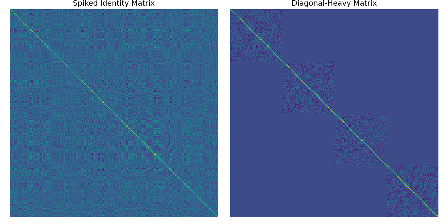
Matrix Construction We empirically verified the theoretical bounds using a modestly large SPSD matrix with dimension \(N=4000\). The goal was to measure performance on four spectral regimes that highlight the strengths and weaknesses of each estimator. Recall that an SPSD matrix \(\mA\) can be diagonalized as \(\mA = \mQ \mD \mQ^\top\) where \(\mD\) is a diagonal matrix of eigenvalues \(\lambda_1 \geq \lambda_2 \geq \ldots \geq \lambda_N \geq 0\) and \(\mQ\) is an orthogonal matrix of eigenvectors. The same Discrete Cosine Transform (DCT) mixing matrix \(\mQ\) discussed in Section 4 is applied as a unitary operation for the basis-oblivious construction of dense test matrices from diagonal eigenvalue matrices \(\mD\). A diagonal-heavy matrix with concentrated blocks along the diagonal is used to evaluate performance on structured sparse matrices.
- Slow Decay (\(\lambda_k \propto k^{-1}\)): The slow decay matrix is more uniform with fewer “heavy-hitters”; the eigenbasis is randomized with DCT.
- Fast Decay (\(\lambda_k \propto k^{-2}\)): The quadratic decay has concentrated spectral energy in the leading eigenvalues; the eigenbasis is randomized with DCT.
- Diagonal-Heavy: A block diagonal matrix with correlated blocks to concentrate \(\|\mA\|_F\) in the diagonal elements, creating a favorable scenario for Rademacher vectors in Hutchinson. A sample matrix of this form is shown in Figure 1.
- Spiked Identity: An identity matrix with a low-rank signal added to create a few large eigenvalues. A sample matrix of this form is shown in Figure 1.
Evaluation Metrics For each of these tasks, the Rademacher and Gaussian variants of Hutchinson and Hutch++ were run for a range of MVP budgets \(m\). The true trace \(\tr(\mA)\) was computed directly for error calculation, and the convergence behavior was recorded. The relative error \(|\tr(\mA) - T|/\tr(\mA)\) is averaged over 50 trials, with the variance shown to \(\pm \frac{1}{2}\sigma\).
6.2 Code and Trials
Algorithm Implementation
Starting with Hutchinson’s estimator, the implementation is straightforward as shown below. The multiple queries are modeled as a matrix-matrix product for efficiency where \(\mV\) is a matrix of \(m\) random vectors as columns. Using the property that the trace can be expressed as a Frobenius inner product, we have:
\[ \begin{align} T_H &= \frac{1}{m} \sum_{j=1}^m \vv_j^\top \mA \vv_j = \frac{1}{m} \sum_{j=1}^m [\mV^\top \mA \mV]_{jj} \\ &= \frac{1}{m} \tr(\mV^\top \mA \mV) \\ &= \frac{1}{m}\langle \mV, \mA \mV \rangle_F = \frac{1}{m}\sum_{i=1}^n \sum_{j=1}^m V_{ij} Y_{ij} , \end{align} \] which is computed by summing the elementwise product of \(\mV\) and \(\mY = \mA \mV\).
The Hutch++ implementation follows the steps outlined in alg. 1 and alg. 2. In this case we optimize the computation step by noting that the projection \((\mI - \mQ \mQ^\top)\) can be applied efficiently without explicitly forming the projection matrix. For the projection matrix \(P = \mI - \mQ \mQ^\top\), we have that \(P = P^\top\) and \(P^2 = P\). Thus for any matrix \(\mG\) the projected MVP can be computed as \(\tr(P \mA P) = \tr(\mA P)\) and so using standard Hutchinson on the residual becomes \[ \tr(P \mA P) = \tr(PA) \approx \langle \mG, P\mA \mG \rangle_F \]
def hutch_plus_plus(A, num_queries, dist="rademacher"):
    """
    Hutch++ with support for Rademacher or Gaussian sketching.

    Args:
        A (ndarray): The input matrix.
        num_queries (int): Total matrix-vector product budget (m).
        dist (str): 'rademacher' or 'gaussian'. Controls the distribution of the
                    sketching matrix Omega and the query split ratio.
    """
    n = A.shape[0]
    m = num_queries

    # 1. construct the sketching matrix based on distribution
    if dist == "rademacher":
        # Rademacher uses m/3 split
        s_queries = max(2, int(m / 3))
        S = np.random.randint(0, 2, size=(n, s_queries)) * 2 - 1
    elif dist == "gaussian":
        # Gaussian uses (m+2)/4 split
        s_queries = max(2, int((m + 2) / 4))
        S = np.random.randn(n, s_queries)
    else:
        raise ValueError("dist must be 'rademacher' or 'gaussian'")

    # 2. Compute the orthonormal basis Q for the sketch AS via QR decomposition
    Y = A @ S
    Q, _ = np.linalg.qr(Y)

    # 3. Compute combination of lowrank trace with the residual hutchinson
    AQ = A @ Q
    tr_low_rank = np.sum(Q * AQ) # Frobenius inner product for trace

    # Remaining queries for residual Hutchinson
    m_rem = m - 2 * s_queries
    if m_rem <= 0:
        return tr_low_rank

    # Sample new Rademacher vectors for residual trace estimation
    G = np.random.randint(0, 2, size=(n, m_rem)) * 2 - 1
    AG = A @ G

    AG_proj = AG - Q @ (Q.T @ AG)  # Project AG onto the orthogonal complement of Q

    # Each column product corresponds to one sample of the residual trace
    tr_res = np.sum(G* AG_proj) / m_rem

    return tr_low_rank + tr_res
For experimentation, a generalized construction method for PSD with different spectral profiles is implemented by sampling eigenvalues from a \(1/n^k\) decay function and applying the discrete cosine transform for mixing. The diagonal-heavy and spiked identity matrices are constructed directly.
Show the code
def generate_dct_rotated_matrix(n, decay_power):
    """
    Constructs A = Q D Q^T SPSD matrix with:
    - D: Diagonal with eigenvalues decaying as 1/k^decay_power
    """
    # 1. Eigenvalues (Diagonal D)
    evals = 1.0 / np.arange(1, n + 1) ** decay_power
    D = np.diag(evals)

    # 2. Construct Q via Randomized DCT
    I = np.eye(n)
    Q_dct = dct(I, type=2, norm="ortho", axis=0)
    signs = np.random.choice([-1, 1], size=n)
    Q = Q_dct * signs[:, np.newaxis]  # Broadcasting to multiply rows

    # 3. Construct A = Q D Q^T
    A = Q @ D @ Q.T

    return A, np.sum(evals)

def generate_clustered_covariance(N, n_clusters=5, cross_talk=0.01):
    """
    Generates a Block Diagonal-ish Matrix (Clustered Correlation).
    - 'n_clusters' dense blocks along the diagonal.
    - 'cross_talk' weak random correlation between blocks.
    """
    block_size = N // n_clusters
    remainder = N % n_clusters

    # Start with noise background (weak cross-talk)
    # Construct as B * B^T to ensure SPSD
    B_noise = np.random.randn(N, max(10, N // 10)) * np.sqrt(cross_talk)
    A = B_noise @ B_noise.T

    # Add dense blocks to diagonal
    current_idx = 0
    for i in range(n_clusters):
        size = block_size + (1 if i < remainder else 0)

        # Create a random dense correlation matrix for this block
        # Spectrum: Linear decay (standard random matrix)
        X_block = np.random.randn(size, size)
        C_block = X_block @ X_block.T

        # Normalize block to have reasonable scale (e.g., max eigenvalue ~ 1)
        C_block /= np.linalg.norm(C_block, 2)

        # Add to the big matrix diagonal
        A[current_idx : current_idx + size, current_idx : current_idx + size] += C_block
        current_idx += size

    return A, np.trace(A)

def generate_spiked_identity(N, rank=50, signal_strength=100.0):
    """
    Generates a 'Spiked Identity' matrix: A = I + U S U^T.
    - N: Size of the matrix.
    - rank: Rank of the low-rank signal.
    - signal_strength: Controls the magnitude of the spikes.


    """
    # 1. Identity (Noise floor)
    A = np.eye(N)

    # 2. Add Low Rank Signal (Spikes)
    # Random subspace U
    U = np.random.randn(N, rank)
    U, _ = np.linalg.qr(U)

    # Eigenvalues for the signal part (decaying)
    evals_signal = np.linspace(signal_strength, signal_strength/10, rank)

    # Update A: A = I + U * diag(S) * U^T
    A += U @ (np.diag(evals_signal) @ U.T)

    true_trace = N + np.sum(evals_signal)
    return A, true_trace
6.3 Results and Discussion
The results are presented below in Figure 2:
Show the code
import time
import numpy as np
import matplotlib.pyplot as plt
import pickle
import os

np.random.seed(42)
N, trials = 5000, 30
query_counts = np.unique(np.geomspace(10, 500, num=10, dtype=int))

# Define datasets (Functions assumed to be defined in a previous cell)
datasets = [
    ("Slow Decay ($1/k$)", generate_dct_rotated_matrix(N, 1.0)),
    ("Fast Decay ($1/k^2$)", generate_dct_rotated_matrix(N, 2.0)),
    ("Clustered Covariance", generate_clustered_covariance(N, n_clusters=20, cross_talk=0.00)),
    ("Spiked Identity ($I + LR$)", generate_spiked_identity(N, rank=50, signal_strength=100.0)),
]

methods = [
    ("Hutch (Rad)",   lambda A, q: hutchinson(A, q, "rademacher"),      "#1f77b4", "o-"),
    ("Hutch (Gauss)", lambda A, q: hutchinson(A, q, "gaussian"),        "#ff7f0e", "s--"),
    ("H++ (Rad)",     lambda A, q: hutch_plus_plus(A, q, "rademacher"), "#2ca02c", "^-"),
    ("H++ (Gauss)",   lambda A, q: hutch_plus_plus(A, q, "gaussian"),   "#9467bd", "d-."),
]

cache_file = "trace_estimation_results.pkl"
run_simulation = not os.path.exists(cache_file)

if run_simulation:
    print("No cache found. Running simulations (this may take a while)...")
    # Data structures to store results
    # We store the raw trial errors to allow for flexible re-plotting of variance/mean
    trial_results = {}
    timing_stats = {}

    for name, (A, true_tr) in datasets:
        trial_results[name] = {}
        timing_stats[name] = {}

        for label, func, _, _ in methods:
            errors = np.zeros((len(query_counts), trials))
            times = np.zeros(len(query_counts))

            for i, q in enumerate(query_counts):
                t_start = time.perf_counter()
                for t in range(trials):
                    est = func(A, q)
                    errors[i, t] = np.abs(est - true_tr) / true_tr
                times[i] = (time.perf_counter() - t_start) / trials # Avg time per query

            trial_results[name][label] = errors
            timing_stats[name][label] = times

    # Bundle everything for pickle
    payload = {
        "trial_results": trial_results,
        "timing_stats": timing_stats,
        "query_counts": query_counts,
        "N": N,
        "trials": trials
    }

    with open(cache_file, "wb") as f:
        pickle.dump(payload, f)
    print(f"Results saved to {cache_file}.")

else:
    with open(cache_file, "rb") as f:
        data = pickle.load(f)

    trial_results = data["trial_results"]
    timing_stats = data["timing_stats"]
    query_counts = data["query_counts"]

# Define style mapping here so you can change colors/markers without re-computing
style_map = {
    "Hutch (Rad)":   {"color": "#1f77b4", "fmt": "o-"},
    "Hutch (Gauss)": {"color": "#ff7f0e", "fmt": "s--"},
    "H++ (Rad)":     {"color": "#2ca02c", "fmt": "^-"},
    "H++ (Gauss)":   {"color": "#9467bd", "fmt": "d-."},
}

fig, axes = plt.subplots(2, 2, figsize=(12, 10))
axes_flat = axes.flatten()

for ax, (name, labels_dict) in zip(axes_flat, trial_results.items()):
    for label, errors in labels_dict.items():
        # Retrieve style
        color = style_map[label]["color"]
        fmt = style_map[label]["fmt"]

        # Calculate statistics from raw trial data
        mu = np.mean(errors, axis=1)
        sigma = np.std(errors, axis=1)

        # Main Plot
        ax.loglog(query_counts, mu, fmt, label=label, color=color, lw=1.5, markersize=4)

        # Confidence Interval (shaded area)
        lower = np.maximum(mu - 0.5 * sigma, 1e-10)
        upper = np.minimum(mu + 0.5 * sigma, 1.0)
        ax.fill_between(query_counts, lower, upper, color=color, alpha=0.1)

    # Reference Complexity Lines
    ax.loglog(query_counts, 1.0 / np.sqrt(query_counts), "k:", label=r"$O(1/\sqrt{m})$", alpha=0.4)
    ax.loglog(query_counts, 1.0 / query_counts, "k-.", label=r"$O(1/m)$", alpha=0.4)

    ax.set_title(name, fontweight='bold')
    ax.set_xlabel("Matrix-Vector Queries (m)")
    ax.set_ylabel("Relative Error")
    ax.grid(True, which="both", ls="-", alpha=0.2)

    if ax == axes_flat[0]: # Legend only on first plot to reduce clutter
        ax.legend(fontsize="small", loc="upper right", frameon=True)

plt.tight_layout()
plt.show()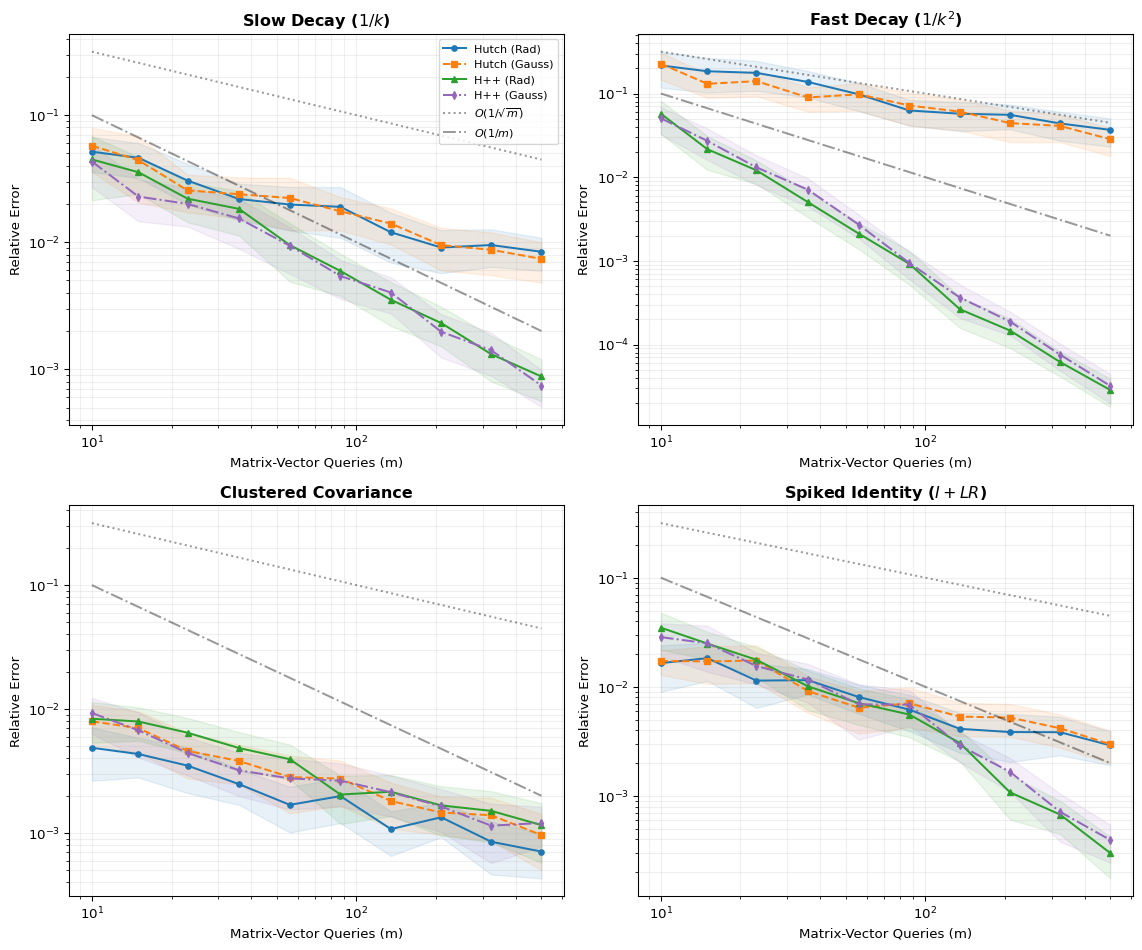
Impact of Decay Rate As expected, the Hutch++ performance gain is most pronounced in a fast decay spectrum, where the low-rank approximation concentrates the MVP budget on the largest contributors to variance in the trace estimate. The difference is accentuated by the log-log scale where Hutch++ quickly attains several orders of magnitude lower error for the same number of MVPs. For slow decays and smaller numbers of queries, the advantage is less pronounced over the standard Hutchinson.
Rademacher vs Gaussian Interestingly, the choice of random variable does not have a significant impact on performance, despite the theoretical bounds and methods to attain them being quite different. Rademacher only shows a clear advantage in the diagonal-heavy regime, where it is able to even outperform the Hutch++ methods. Note that the Gaussian variant of Hutch++ only uses Gaussian variables for the sketching matrix, while the residual estimation still uses Rademacher vectors.
Convergence Slope In all regimes, the performance follows the slope of the bounds quite closely, indicating that the theoretical analysis is tight. In the fast decay regime, Hutch++ outperforms the theoretical bounds, which make no assumptions on the rate of decay. Note that the error is compared against the number of queries; the inverse relationship is thus \(O(1/m)\), giving a slope of -1 on the log-log plots, while Hutchinson has a slope of -0.5 as expected from the \(O(1/\sqrt{m})\) dependence. The slope of Hutch++ in fast decay is even steeper, showing the adaptive leveraging of the spectrum.
Wall Clock Time The focus of this work has been on the bounds and theoretical convergence for trace estimation. However, factorization steps such as the \(QR\) decomposition and generation of random vectors add time to the overhead. To get a better sense of practical performance with time as a resource instead of MVPs, a wall clock time comparison is shown in Figure 3. The time taken scales linearly with the queries, indicating that the MVP query bounds are roughly equivalent to the time bounds, as claimed by Meyer et al. (2021).
Show the code
fig, axes = plt.subplots(2, 2, figsize=(12, 10))
axes_flat = axes.flatten()

# Iterate through datasets using the keys in trial_results
for ax, (name, labels_dict) in zip(axes_flat, trial_results.items()):
    for label, errors_matrix in labels_dict.items():
        color = style_map[label]["color"]
        fmt = style_map[label]["fmt"]

        mu_error = np.mean(errors_matrix, axis=1)
        avg_time = timing_stats[name][label]

        # Plot Time (X) vs. Error (Y)
        ax.loglog(avg_time, mu_error, fmt, label=label, color=color, lw=2, markersize=6)

    ax.set_title(f"Efficiency: {name}", fontweight='bold')
    ax.set_xlabel("Average Wall-Clock Time (seconds)")
    ax.set_ylabel("Relative Error")
    ax.grid(True, which="both", ls="-", alpha=0.3)

    # Legend on the first subplot
    if ax == axes_flat[0]:
        ax.legend(fontsize="small", loc="upper right", frameon=True)

plt.tight_layout()
plt.suptitle("Efficiency Frontier: Accuracy vs. Computational Cost", fontsize=16, y=1.02)
plt.show()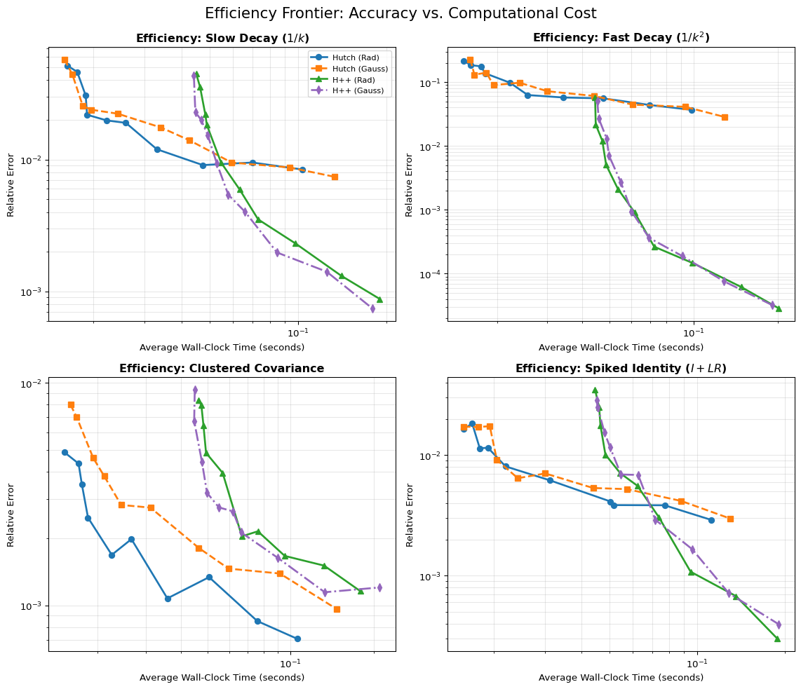
7 Conclusion
7.1 Future Work and Applications
One impactful application for matrix-free implicit trace estimation with Hutch++ is in the training of continuous normalizing flows and diffusion models. Recent work by Liu et al. (2025) directly leverages the Hutch++ estimator to improve divergence-based likelihood estimation. The process of \(QR\) decomposition is modified to share the same decomposition of \(Q\) across multiple time steps of the integration, reducing the overhead cost of the method without sacrificing too much performance, as the top eigenbasis of the Jacobian does not change significantly over small time intervals of the normalizing flow. To this effect, the problem above can be seen as a dynamic trace estimation problem where the implicit matrices are strongly correlated. Woodruff et al. (2022) addresses this optimization, building upon the original Hutch++ framework to improve the query complexity while also proving new lower bounds for Hutchinson, resolving the open question of tightness for original Hutchinson in Meyer et al. (2021).
7.2 Summary
This work presents a review of randomized algorithms for implicit trace estimation with a focus on SPSD matrices. The progression of analysis from variance in Hutchinson’s original Rademacher estimator, to the Chernoff-style bounds of Avron and Toledo (2011), to the optimal Hutch++ algorithm of Meyer et al. (2021) with provable lower bounds and optimality is presented. The progression of authorship and style is notable, with each work contributing further to a broad understanding of optimal implicit trace estimation in many settings. Numerical experiments confirm the theory, showing that Hutch++ is both theoretically and practically superior to Hutchinson in all but the most diagonal-heavy cases. Finally, the application of Hutch++ to generative AI models such as continuous normalizing flows and diffusion models is discussed, demonstrating the relevance of these methods to modern machine learning and research in this area.
The technique of adaptive variance reduction by isolating the top contributors to variance and attributing more resources to them is a powerful idea that we may expect to have further applications in randomized numerical linear algebra and beyond. The first step to many problems is identifying the nature of the problem itself, which the low-rank approximation step of Hutch++ effectively does, providing a provably optimal method for implicit trace estimation.
8 Appendix
Stronger Bound for \(T_{GM}\)
Avron and Toledo (2011) do much better starting with the moment generating function (MGF) of the \(\chi^2\) distribution to derive a Chernoff-style bound. Taking \(Z=m T_{GM} = \sum_{i=1}^N \lambda_i X_i\) where \(X_i \sim \chi^2_m\).
Lemma 2 Let \(X \sim \chi^2_m\). Then the moment generating function of \(X\) is \[ M_{X}(t) = (1 - 2t)^{-m/2}, \quad t < \frac{1}{2}. \]
Definition 4 (Elementary Symmetric Polynomial) The \(s\)-th elementary symmetric polynomial of variables \(\lambda_1, \ldots, \lambda_N\) is defined as \[ e_s(\lambda_1, \ldots, \lambda_N) := \sum_{S \subseteq \{\lambda_1,\ldots,\lambda_N\}, |S|=s} \prod_{\lambda \in S} \lambda. \]
Lemma 3 (Elementary symmetric polynomial bound) Let \(\lambda_1,\ldots,\lambda_N \ge 0\). Then for all \(s \ge 2\), \[ e_s(\lambda) \le \frac{1}{s!}\left(\sum_{i=1}^N \lambda_i\right)^s = \frac{1}{s!}\,\tr(\mA)^s. \]
Proof. By the definition, \(e_s\) gives all products of \(s\) distinct \(\lambda_i\)’s, that is with multiplicity one. On the other hand, expanding \(\left(\sum_{i=1}^N \lambda_i\right)^s\), gives each distinct multiplicity one term \(s!\) times due to permutations being included in the expansion. In addition there are terms with multiplicities higher than one which are not in \(e_s\). Thus we have \[ \left(\sum_{i=1}^N \lambda_i\right)^s = s! \cdot e_s(\lambda_1, \ldots, \lambda_N) + \text{(higher multiplicities)} \] \[ \geq s! \cdot e_s(\lambda_1, \ldots, \lambda_N) \quad \text{ since } \lambda_i \geq 0 \] \[ e_s(\lambda_1, \ldots, \lambda_N) \leq \frac{1}{s!}\left(\sum_{i=1}^N \lambda_i\right)^s \quad \square \]
To prove the tighter bound for \(T_{GM}\), we derive the MGF for \(Z\) using the independence of the \(X_i\)’s and the scaling property of MGFs. \[ \begin{align} M_{Z}(t) &= \mathbb{E}\left[e^{t Z}\right] \\ &= \prod_{i=1}^N M_{X_i}(\lambda_i t) \\ &= \prod_{i=1}^N (1 - 2 \lambda_i t)^{-m/2}, \quad t < \frac{1}{2 \max_i \lambda_i}. \end{align} \] The next step is to take the expansion of the product and bound the terms, noting that \(\lambda_i \geq 0\) for SPSD matrices. Using the definition of the elementary symmetric polynomials, we have \[ M_{Z}(t) = \left(1-2 t \tr(\mA) + \sum_{s=2}^{N}(-2)^st^s e_s(\lambda_1, \ldots, \lambda_N) \right)^{-m/2} \] Using Lemma 3 to bound the elementary symmetric polynomials, we have \[ \left| \sum_{s=2}^{N}(-2)^st^s e_s(\lambda_1, \ldots, \lambda_N) \right| \leq \sum_{s=2}^{N} 2^s |t|^s \frac{1}{s!} \tr(\mA)^s \le \sum_{s=2}^{N} \left(2 t \tr(\mA)\right)^s \] Setting \(t_0 = \frac{\epsilon}{4 \tr(\mA)(1+\epsilon/2)}\) ensures that \(t_0 < \frac{1}{2 \max_i \lambda_i}\) and the MGF is valid. Recalling that for a geometric series \(\sum_{s=2}^N r^s \leq \sum_{s=2}^\infty r^s = \frac{r^2}{1-r}\) for \(|r|<1\), then we have \[ \left| \sum_{s=2}^{N}(-2)^{s}t_0^{s} e_s(\lambda_1, \ldots, \lambda_N) \right| \leq \left(\frac{\epsilon}{2(1+\epsilon/2)}\right)^2 \left(1 - \frac{\epsilon}{2(1+\epsilon/2)}\right)^{-1} = \frac{\epsilon^2}{4(1+\epsilon/2)} \]
The proof is then completed using Markov’s inequality on the MGF shown in brief form here: \[ \begin{align} \Pr\left[ T_{GM} \geq (1+\epsilon) \tr(\mA) \right] &= \Pr\left[ Z \geq m(1+\epsilon) \tr(\mA) \right] \\ &= \Pr\left[ \exp({t_0 Z}) \geq \exp({t_0 m(1+\epsilon) \tr(\mA)}) \right] \\ &\leq M_{Z}(t_0)\exp\left({-t_0 m(1+\epsilon) \tr(\mA)}\right) \\ & \leq \exp\left(-m\epsilon^2/20\right). \end{align} \] The full proof is given in Avron and Toledo (2011, Theorem 5.2). The same result is applied to the lower tail, with a union bound over both failure \(\delta/2\) events giving the final result that for an \((\epsilon, \delta)\)-approximation we require.
References
Ailon, Nir, and Bernard Chazelle. 2006. “Approximate Nearest Neighbors and the Fast Johnson-Lindenstrauss Transform.” Proceedings of the Thirty-Eighth Annual ACM Symposium on Theory of Computing (New York, NY, USA), STOC ’06, 557–63. https://doi.org/10.1145/1132516.1132597.
Avron, Haim, and Sivan Toledo. 2011. “Randomized Algorithms for Estimating the Trace of an Implicit Symmetric Positive Semi-Definite Matrix.” J. ACM 58 (2): 8:1–34. https://doi.org/10.1145/1944345.1944349.
Harvey, Nicholas J. A. 2021. A Second Course in Randomized Algorithms. University of British Columbia, Course Textbook Draft. https://www.cs.ubc.ca/~nickhar/Book2.pdf.
Hu, Zheyuan, Zekun Shi, George Em Karniadakis, and Kenji Kawaguchi. 2024. “Hutchinson Trace Estimation for High-Dimensional and High-Order Physics-Informed Neural Networks.” Computer Methods in Applied Mechanics and Engineering 424: 116883. https://doi.org/https://doi.org/10.1016/j.cma.2024.116883.
Hutchinson, M. F. 1990. “A Stochastic Estimator of the Trace of the Influence Matrix for Laplacian Smoothing Splines.” Communications in Statistics - Simulation and Computation 19 (2): 433–50. https://doi.org/10.1080/03610919008812866.
Liu, Xinyang, Hengrong Du, Wei Deng, and Ruqi Zhang. 2025. “Optimal Stochastic Trace Estimation in Generative Modeling.” arXiv Preprint arXiv:2502.18808.
Meyer, Raphael A., Cameron Musco, Christopher Musco, and David P. Woodruff. 2021. Hutch++: Optimal Stochastic Trace Estimation. arXiv. https://doi.org/10.48550/arXiv.2010.09649.
Musco, Cameron, and Christopher Musco. 2020. Projection-Cost-Preserving Sketches: Proof Strategies and Constructions. https://arxiv.org/abs/2004.08434.
Pearlmutter, Barak A. 1994. “Fast Exact Multiplication by the Hessian.” Neural Computation 6 (1): 147–60. https://mural.maynoothuniversity.ie/id/eprint/5501/.
Song, Yang, Sahaj Garg, Jiaxin Shi, and Stefano Ermon. 2019. “Sliced Score Matching: A Scalable Approach to Density and Score Estimation.” Conference on Uncertainty in Artificial Intelligence. https://api.semanticscholar.org/CorpusID:158047026.
Ubaru, Shashanka, and Yousef Saad. 2018. “Applications of Trace Estimation Techniques.” In High Performance Computing in Science and Engineering, edited by Tomáš Kozubek, Martin Čermák, Petr Tichý, et al. Springer International Publishing.
Woodruff, David P. 2014. “Sketching as a Tool for Numerical Linear Algebra.” Foundations and Trends® in Theoretical Computer Science 10 (1-2): 1–157. https://doi.org/10.1561/0400000060.
Woodruff, David P., Fred Zhang, and Qiuyi (Richard) Zhang. 2022. “Optimal Query Complexities for Dynamic Trace Estimation.” Proceedings of the 36th International Conference on Neural Information Processing Systems (Red Hook, NY, USA), NIPS ’22.