Synthetic Geology
A talk on the promise of using simulation and generative AI as a learned prior for 3D geological inversion
Links: - Paper (JGR) - Preprint (arXiv) - Geological Simulation Engine (GitHub) - Generative Model (GitHub)
1 Introduction
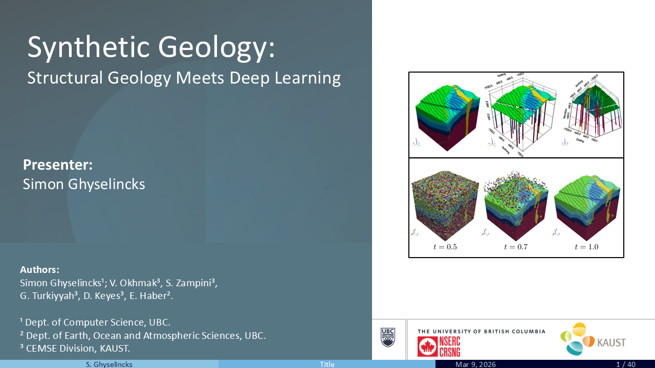
I’m Simon Ghyselincks, a PhD-track graduate student at UBC, co-advised by Eldad Haber (Earth, Ocean and Atmospheric Sciences) and Evan Shelhamer (Computer Science). My research is interdisciplinary, sitting at the intersection of mathematics, computer science, and earth science. This talk presents work from a recently published paper, “Synthetic Geology: Structural Geology Meets Deep Learning” (Ghyselincks et al. 2025), done in collaboration with coauthors at KAUST and supported by NSERC.

The talk is organized into three parts: an Introduction motivating the problem of geological inversion and why deep learning is a promising tool; Simulation Methods covering how we generate diverse 3D models using the GeoGen framework; and Generative Modeling introducing probabilistic machine learning with conditional and unconditional flow matching for ensemble sampling.


2 GeoGen Synthetic Dataset


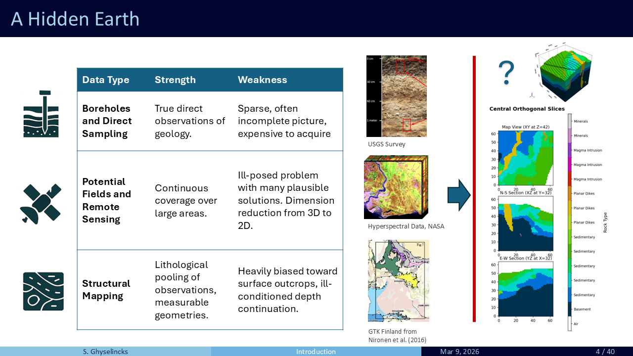
Structural geology examines the distribution of rocks and strata within the Earth’s crust. Generating full-scale 3D geological models can be costly. Existing tools include GemPy (Varga et al. 2019) (shown with a forward model for simulated temperature based on conductivity) and the Noddy modeling kit with the Noddyverse set of randomized models (Jessell et al. 2022).

Our dataset is built as a geological computer and instruction set, with a layer of automated randomization on top. The pipeline starts with a modeling framework, uses random variables to sample geological events, applies randomized event sequencing for variety, and parallelizes through the PyTorch framework.

The stages of model computation:
- Form an empty rectangular meshgrid
- Reverse the mesh through geological time
- Apply initial strata
- Forward the mesh back to the present
Complexity is built through a chain of multiple transformations and depositions, a computational history. The point cloud of sample points is typically most deformed at the beginning of the history sequence and unfolds back to a regular tensor shape as deposits, unconformities, and intrusions are added. This ensures we always end up with a uniform mesh in the present-day sample.

The framework removes the need to specify spatial coordinates to the machine learning model, which learns spatial distributions based on voxel positions in the final mesh.

Geowords are high-level generator classes that bridge the gap between raw probability and geological meaning. They describe events such as a dike cluster or a complex fold in terms of correlated random variables for their parameters. For example, Fold, Fault, and Shear events have distributions over amplitude, direction, and rake. The amplitude is correlated to the period, so parameters are assembled in a structured way to sample plausible geological events.

We generate diverse instruction sets for randomized geology by varying the order of operations and the number of events in a history.

Event sequencing uses Markov sampling: the \(n\)th event type is drawn based on event \((n-1)\) using transition probabilities. An early termination token creates variable-length geologies where the number of operations represents geological history. Young oceanic crust undergoes limited transforms, while aged continental crust is much more highly deformed.

The full pipeline offers:
- Unlimited samples: generate on-the-fly
- Zero disk storage: no pre-computed dataset needed
- Customizable: adjust parameters and geological event distributions
Models generate quickly (~5-10 seconds on a laptop). Samples generate on the CPU while batches process on the GPU.

Limitations:
- Model fidelity: the fidelity of synthetic data to true geology needs further work. Greater expertise from geologists, more features and realism will improve downstream applications.
- Matching forward observations: the observable parts of the model (e.g., surface) should match real-world surface data. Automated tuning of simulation parameters is a topic of recent research from the KAUST collaboration.
3 Generative Modeling: Flow Matching


Now that we have a simulated synthetic dataset, we look at training a generative AI model for categorical data.

Starting with the classical inverse problem: given a model \(\mathbf{m}\) with forward data \(\mathbf{d}\) and Gaussian measurement noise \(\epsilon\):
\[\mathbf{Am} + \epsilon = \mathbf{d}\]
Applying Bayes’ rule and maximizing the posterior \(P(\mathbf{m}|\mathbf{d})\) yields the MAP estimate. Taking the negative log maps this into a minimization:
\[\phi(\mathbf{m}) = \frac{1}{2}\|\mathbf{Am} - \mathbf{d}\|^2 + \alpha R(\mathbf{m})\]
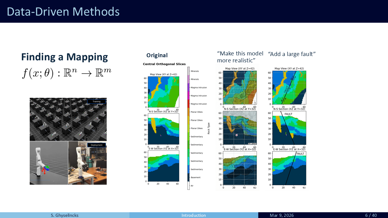
with a misfit term from the noise and a prior (regularization) from our belief about geology. Generative AI targets this probability directly, allowing exploration of the probability space of likely models rather than a single MAP estimate, a probabilistic exploration of the null space of the inverse problem.

Solution: Learn a velocity field that creates a probability flow from a simple (Gaussian) distribution to the target. Taking derivatives avoids the intractable integral (Lipman et al. 2024).
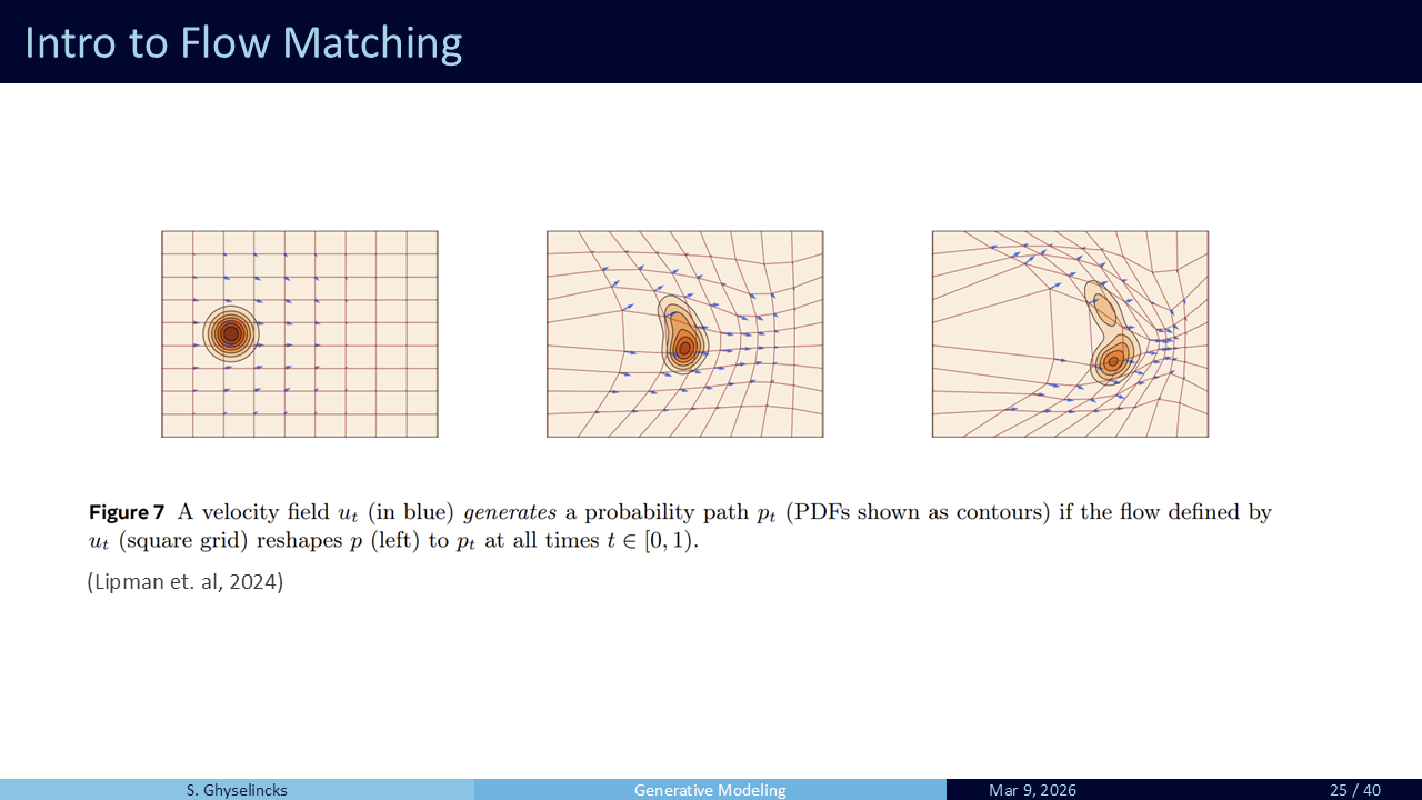
A velocity field \(u_t\) (in blue) generates a probability path \(p_t\) if the flow defined by \(u_t\) reshapes \(p\) (source) to \(p_t\) at all times \(t \in [0, 1)\) (Lipman et al., 2024). The model does not need normalization because it only learns a flow field, not the actual distribution.

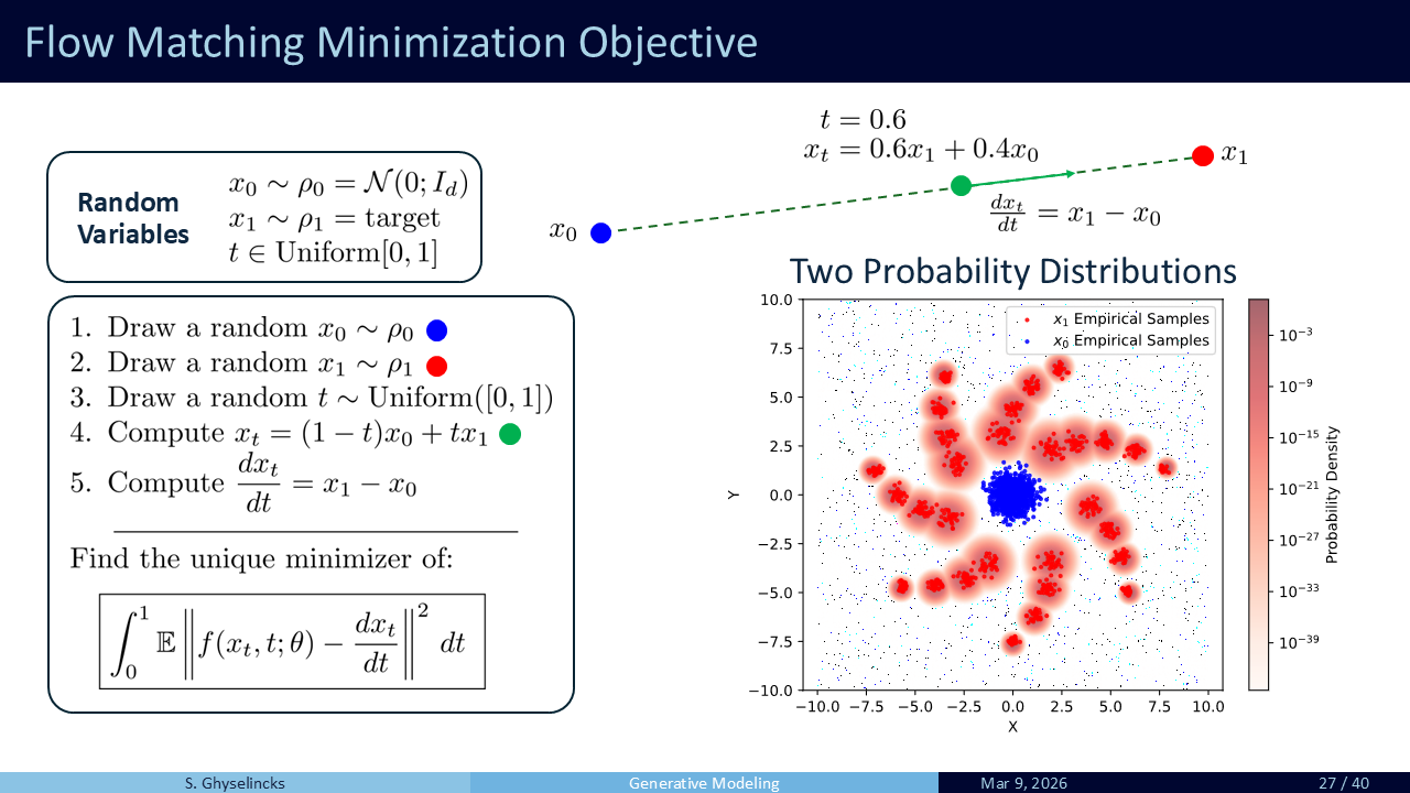
General Framework: We minimize the difference between the true velocity and our estimator model \(\mathbf{v}\) across all pairings and time:
\[\min_{\theta} \frac{1}{2} \mathbb{E}_{t,\mathbf{z},\mathbf{m}} \|\mathbf{v}(\mathbf{m}_t, t; \boldsymbol{\theta}) - \mathbf{v}_t\|_2^2\]
The network randomly samples pairings from both distributions and times, receiving current position and time. Conditional information can also be passed, so called conditional flow matching.
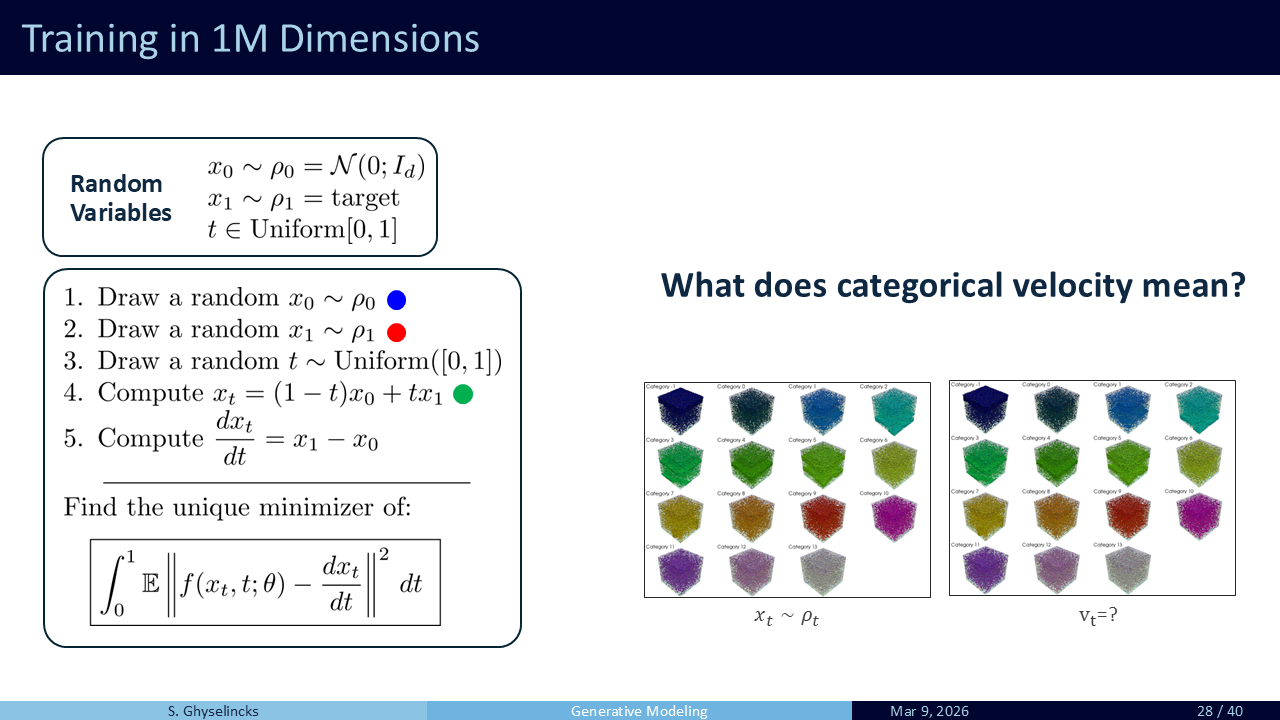
For categorical lithology, we need to embed discrete categories into a continuous space to define categorical velocity. The details are in the paper.

At inference time, we generate new samples by sampling the learned the flow of probability from \(x_0 \sim \rho_0\) to \(x_1 \sim \rho_1\) using an ODE integrator.

Beyond the unconditional prior, we learn the conditional posterior \(P(\mathbf{m}|\mathbf{d})\). Both models and forward data are generated from the simulator. The conditional loss adds a data-fidelity term:
\[\mathcal{L}_{\text{cond}} = \|\hat{\mathbf{v}}(\mathbf{m}_t, \mathbf{d}, t; \boldsymbol{\xi}) - \mathbf{v}_t\|_2^2 + \lambda \cdot t \cdot \|\hat{\mathbf{d}} - \mathbf{d}\|_2^2\]
Note that the data-fidelity term is weighted by time, so the model learns to reconstruct the data at all times, but with more emphasis on later times when the model is closer to the target distribution. This gives freedom and flexibility in the early stages of generation with a tighter requirement to match the forward data as the model approaches the target distribution.

The machine learning model is a 3D U-Net with convolutional layers, attention blocks, multiple scales, and time + data embeddings.

The full training architecture incorporates time embedding, conditional data embedding through skip connections, self-attention, and gradient backpropagation through the conditional loss.
4 Results


Unconditional Generative Model:
The model learns to generate diverse geological structures across 14 rock-type categories from pure noise.

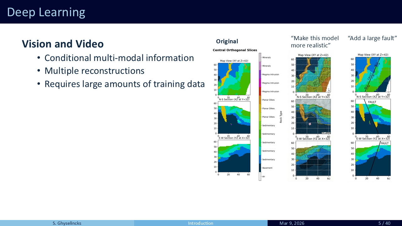
Conditional Generative Model: Given surface and borehole data, the model produces multiple plausible 3D reconstructions.

By creating an ensemble of conditional samples from \(P(\mathbf{m}|\mathbf{d})\), we can estimate feature extent using votes from each voxel. This provides uncertainty quantification on geological features such as dike geometry and extent.
5 Conclusions and Future Work


- Interpretability: Using attention weighting and sensitivity analysis to explain why the model reconstructed a specific feature based on conditional data. Sensitivity analysis and UQ to understand the robustness of solutions.
- Multimodal Integration: Using the backbone network to ingest new data types through latent input fine-tuning.
- Probability Scoring: Finding ways to score samples from a generative AI to quantify which models are more likely.

6 References

